Amazon Warehouse
Goal
The objective of this exercise is to implement the logic that allows a logistics robot to deliver shelves to the required place by making use of the location of the robot. The robot is equipped with a map and knows its current location in it. The main objective will be to find the shortest path to complete the task.
Frequency API
import Frequency- to import the Frequency library class. This class contains the tick function to regulate the execution rate.Frequency.tick(ideal_rate)- regulates the execution rate to the number of Hz specified. Defaults to 50 Hz.
Robot API
This exercise now supports ROS 2-direct implementation in addition to the original HAL-based approach. Below you’ll find the details for both options.
HAL-based Implementation
Python
import HAL- to import the HAL (Hardware Abstraction Layer) library class. This class contains the functions that send and receive information to and from the Hardware (Gazebo).import WebGUI- to import the WebGUI (Web Graphical User Interface) library class. This class contains the functions used to view the debugging information, like image widgets.-
Gazebo Harmonic support
This exercise can also run in Gazebo Harmonic, which is the recommended simulator as Gazebo Classic is being progressively deprecated.
When running the exercise in Gazebo Harmonic, the following imports must be used:
import HAL2 as HAL
import WebGUI2 as WebGUI
Note: Both modules must include the 2 suffix. Using only one of them (HAL2 with WebGUI, or HAL with WebGUI2) will not work correctly
HAL.getPose3d()- returns x, y and theta components of the robot in world coordinates. The function returns an x,y based in this axis reference, with (0,0) next to the robot spawn in Warehouse 1:

HAL.getSimTime()- returns simulation time.# simulation time in second sec = HAL.getSimTime().sec + HAL.getSimTime().nanosec / 1000000000HAL.setV()- to set the linear speed.HAL.setW()- to set the angular speed.HAL.lift()- to lift the platform.HAL.putdown()- to put down the platform.WebGUI.showPath(array)- shows a path on the map. The parameter should be a 2D array containing each of the points of the path.WebGUI.getMap(url)- returns a numpy array with the image data in a 3 dimensional array (R, G, B) of values between 0-1. The URLs of the worlds are in the Supporting information section.WebGUI.showNumpy(mat)- Displays the matrix sent. Accepts an uint8 numpy matrix, values ranging from 0 to 127 for grayscale and values 128 to 134 for predetermined colors (128 = red; 129 = orange; 130 = yellow; 131 = green; 132 = blue; 133 = indigo; 134 = violet).
To reset the map to the original state you can use the next function with orig_map being the original map:
def reset_map(orig_map):
    rows, cols, _ = orig_map.shape
    old_map = np.zeros((rows, cols), dtype=np.uint8)
    for i in range(rows):
        for j in range(cols):
            old_map[i, j] = np.average(orig_map[i, j]) * 127

    WebGUI.showNumpy(old_map)
To draw more complex shapes you can use the following opencv2 functions with mat being the matrix you will use to call WebGUI.showNumpy(mat):
- Draw a line:
cv2.line(mat, (start_x, start_y), (end_x, end_y), color, thickness) - Draw a circle:
cv2.circle(mat, (center_x, center_y), radius, color, thickness) - Draw a rectangle:
cv2.rectangle(mat, (start_x, start_y), (end_x, end_y), color, thickness) - Write text:
image = cv2.putText(mat, text, (start_x, start_y), font, fontScale, color, thickness, cv2.LINE_AA)
See the example below on how to use them:
    rows, cols, _ = orig_map.shape
    mat = np.zeros((rows, cols), dtype=np.uint8)

    cv2.circle(mat, (100, 100), 40, 50, 5)
    cv2.line(mat, (100, 100), (200, 200), 129, 2)
    cv2.rectangle(mat, (100, 100), (200, 200), 128, 2)
    cv2.putText(mat, "Text", (200, 200), cv2.FONT_HERSHEY_SIMPLEX, 1, 129, 2, cv2.LINE_AA)
    WebGUI.showNumpy(mat)
ROS 2-direct Implementation
ROS 2 Topics
Use standard ROS 2 topics for direct communication with the simulation and the WebGUI.
/amazon_robot/cmd_vel- Publish to this topic to set both linear and angular velocities. Message type:geometry_msgs/msg/Twist/amazon_robot/odom- Subscribe to this topic to receive the current pose of the robot. Message type:nav_msgs/msg/Odometry/amazon_robot/scan- Subscribe to this topic to receive the 2D laser data. Message type:sensor_msgs/msg/LaserScan/platform/cmd_vel- Publish to this topic to control the lifting platform. Positive values lift the platform (5.0) and negative values (-5.0) lower it. Message type:std_msgs/msg/Float64
For WebGUI debugging:
/webgui/path- Publish the planned path so it can be displayed in the WebGUI. Message type:std_msgs/msg/String. QoS:TRANSIENT_LOCAL(depth 1)/webgui/image- Publish a debug image for visualization in the WebGUI. Message type:sensor_msgs/msg/Image. QoS:TRANSIENT_LOCAL(depth 1)
Python
Note: Ensure this import is included in your script to access the Web GUI functionalities.
import WebGUI - to enable the Web GUI for visualizing camera images.
To have frequency control you need to use standard ROS 2 mechanisms to manage loop timing:
rclpy.spin()- Event-driven execution using callbacks.rclpy.spin_once()- Single-step processing, often with custom timers.rclpy.Rate()- Loop-based frequency control.
Note
WebGUI already initializes rclpy internally, so this should be taken into account when building a direct ROS 2 solution.
Gazebo Harmonic tools
In Gazebo Harmonic it is possible to manually place the robot in the world using the Entity Tree and Transform Control tools. This can be useful for inspecting world coordinates and verifying the alignment between the simulation and the map used in the exercise, which is particularly helpful when working with the coordinate transformations described in Conversion From 3D to 2D.
This is the standard way to manually manipulate entities in Gazebo Harmonic through the graphical interface.
To enable this feature:
- Open the three-dot menu in Gazebo Harmonic.
- Open the plugin selector.
- Enable:
- Entity Tree
- Transform Control
Once enabled, select the robot in the Entity Tree. The Transform tool will display the manipulation axes directly on the robot model. Using these axes, the robot can be translated in the world to inspect positions and coordinates.

Supporting information
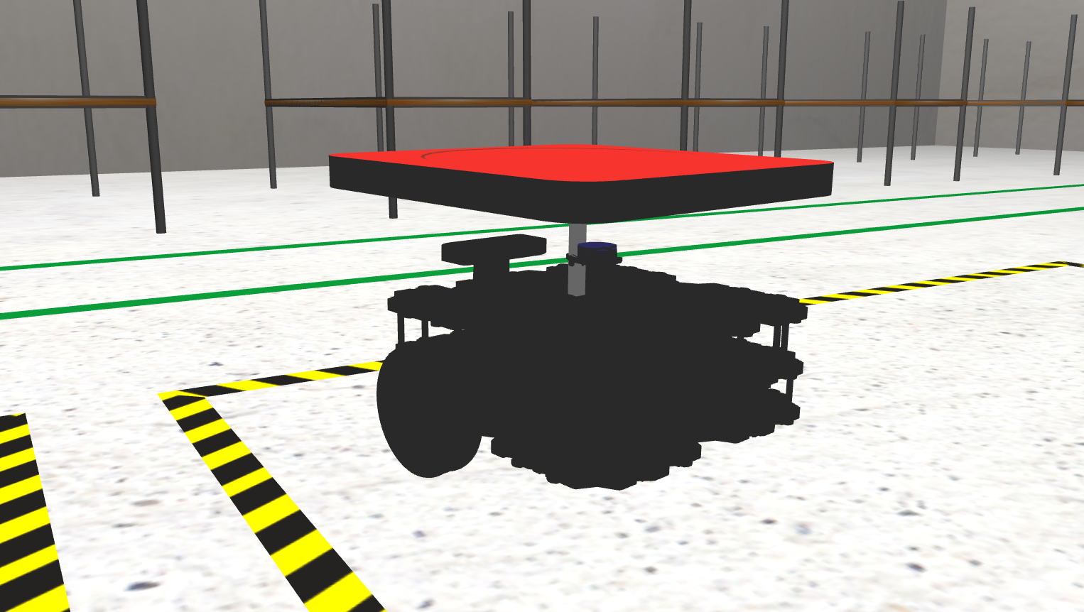
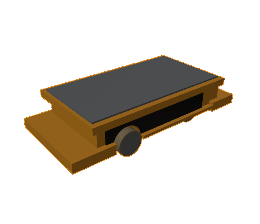
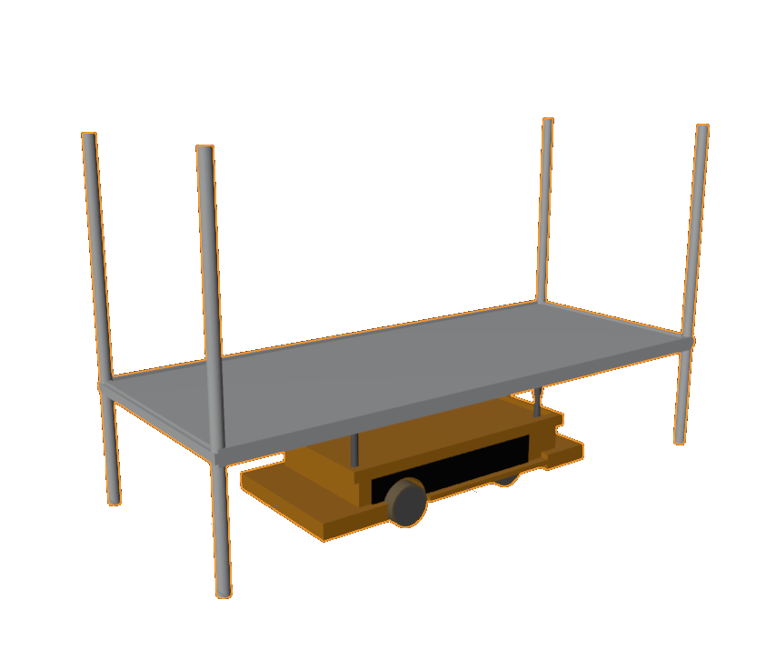
There are two robots to choose from:
Holonomic robot:
- The robot size is 0.3 meters long and 0.3 meters wide.
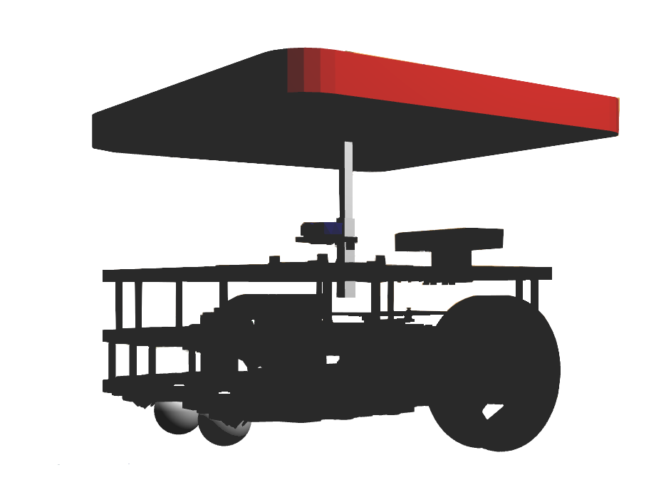
Ackermann robot:
- The robot size is 0.72 meters long and 0.32 meters wide.
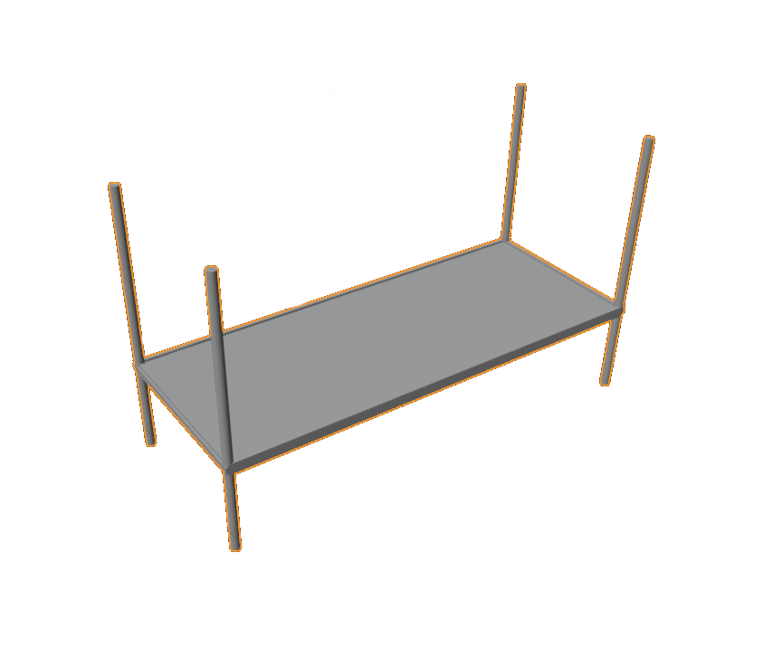
- You can get the robot’s mesh files from there:
- Only robot: /resources/exercises/amazon_warehouse/meshes/robot/ackermann_robot.dae
- Robot lifting a shelf: /resources/exercises/amazon_warehouse/meshes/robot/ackermann_robot_lifting_shelf.dae
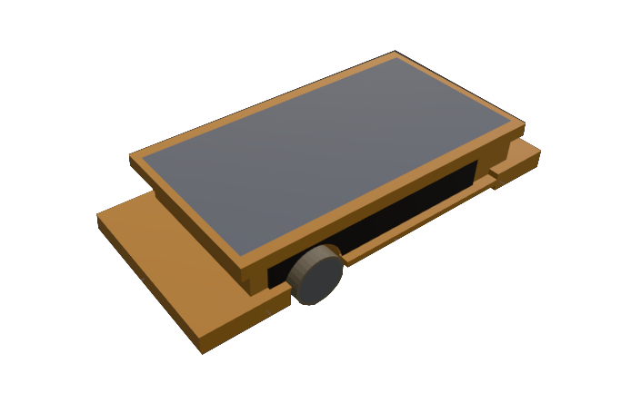
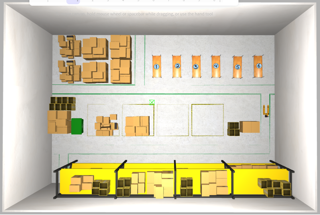
There are two warehouses to choose from:
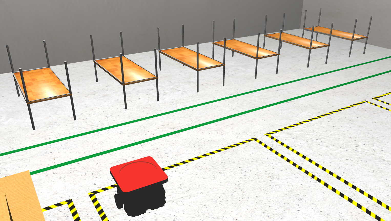
Warehouse 1:
- The warehouse size is 20.62 meters long and 13.6 meters wide.
- The shelves coordinates from 1 to 6 are: (3.728, 0.579), (3.728, -1.242), (3.728, -3.039), (3.728, -4.827), (3.728, -6.781), (3.728, -8.665).
- You can get the warehouse’s map from there: /resources/exercises/amazon_warehouse/images/map.png
- You can get the warehouse’s mesh file from there:
- Warehouse without shelves: /resources/exercises/amazon_warehouse/meshes/world/warehouse1/warehouse1.dae
- Shelf 1: /resources/exercises/amazon_warehouse/meshes/world/warehouse1/shelf1.dae
- Shelf 2: /resources/exercises/amazon_warehouse/meshes/world/warehouse1/shelf2.dae
- Shelf 3: /resources/exercises/amazon_warehouse/meshes/world/warehouse1/shelf3.dae
- Shelf 4: /resources/exercises/amazon_warehouse/meshes/world/warehouse1/shelf4.dae
- Shelf 5: /resources/exercises/amazon_warehouse/meshes/world/warehouse1/shelf5.dae
- Shelf 6: /resources/exercises/amazon_warehouse/meshes/world/warehouse1/shelf6.dae
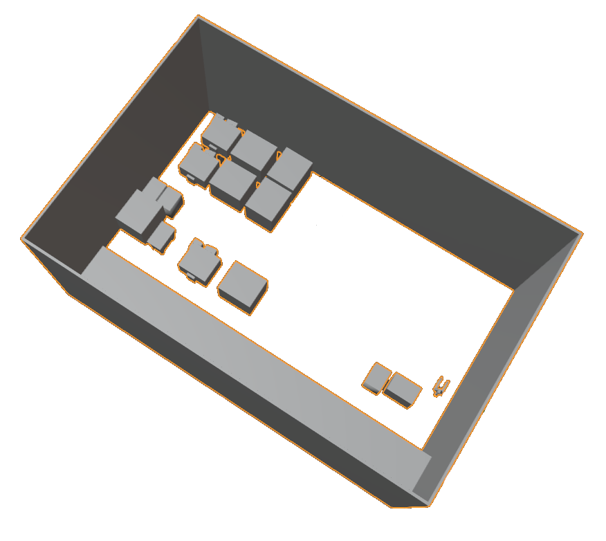
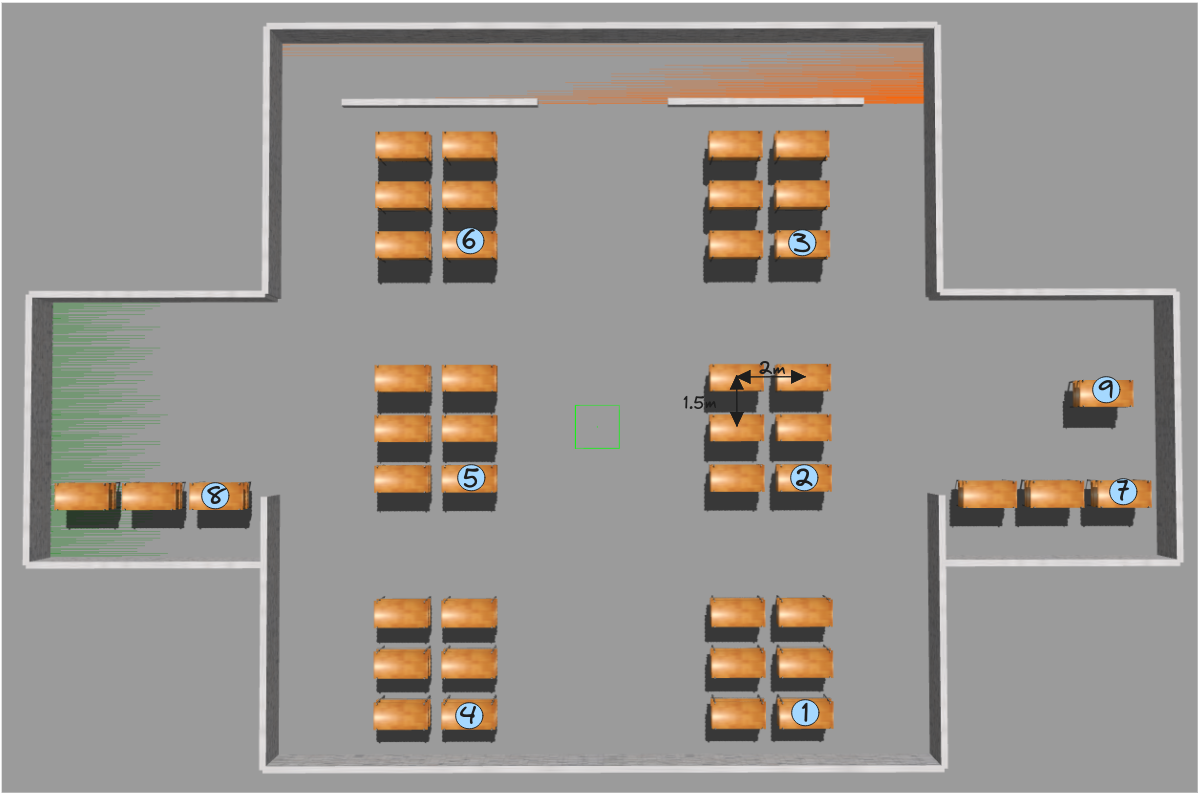
Warehouse 2:
- The warehouse size is 34 meters long and 22 meters wide.
- The shelves coordinates from 1 to 9 are: (-8.5, -6.0), (-1.5, -6.0), (5.5, -6.0), (-8.5, 4.0), (-1.5, 4.0), (5.5, 4.0), (-1.0, -15.5), (-2, 11.5), (1.0, -15.0).
- The separation distance between two neighboring shelves is 2 m on the x axis and 1.5 m on the y axis.
- You can get the warehouse’s map from there: /resources/exercises/amazon_warehouse/images/map_2.png
Theory
This exercise is a motion planning problem. Jderobot Academy already has an exercise dedicated to this, which I’d definitely recommend the readers to check out, so the challenge in this exercise isn’t to implement a motion planning algorithm but learning to use the OMPL (Open Motion Planning Library) for our purpose.
Open Motion Planning Library
OMPL is a library for sampling-based motion planning, offering many state-of-the-art planning algorithms such as PRM, RRT, KPIECE, etc.
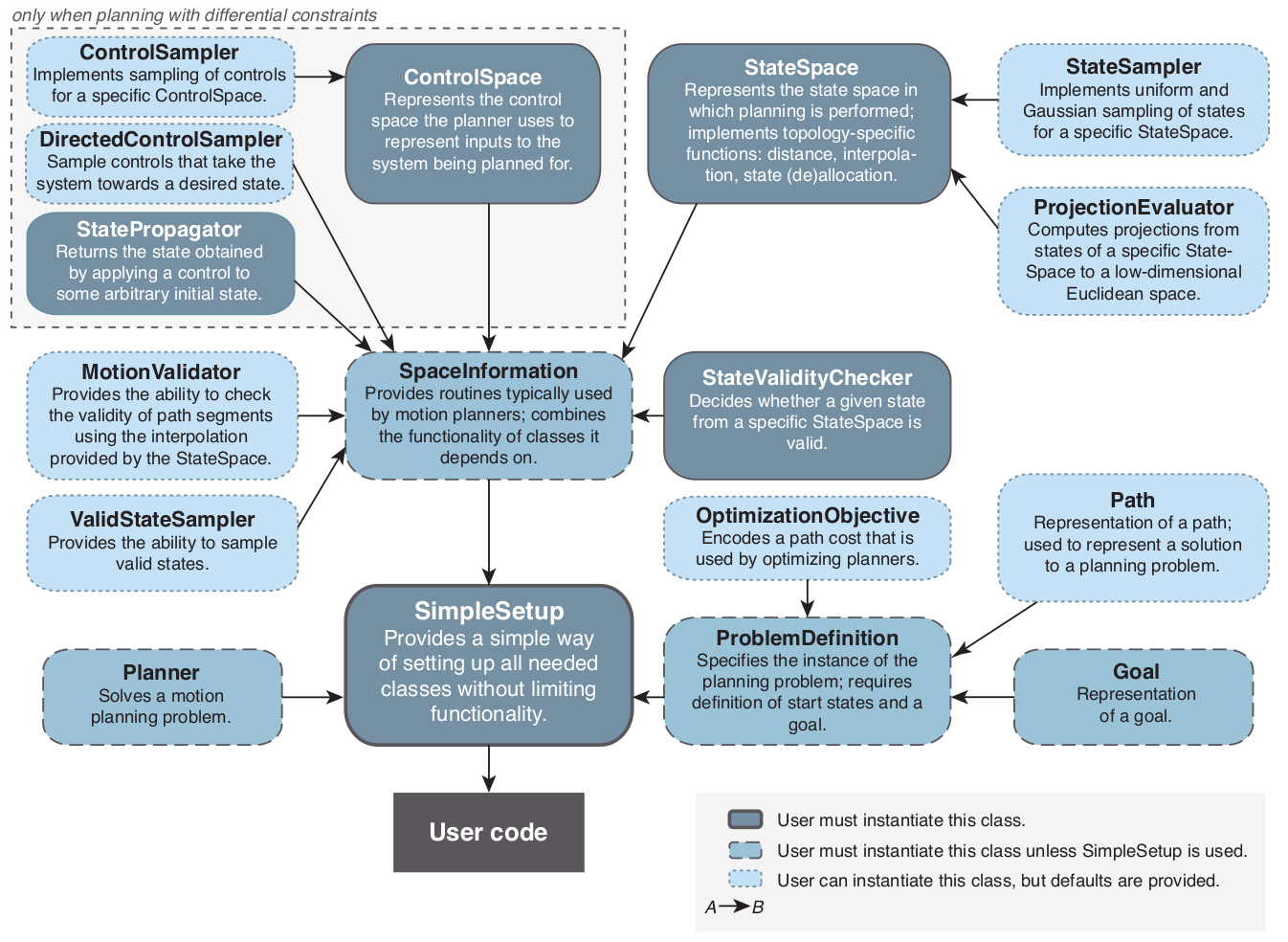
As you can see in the diagram above, some key components of OMPL are:
- State Space defines the possible configurations that a robot can have. For example:
- RealVectorStateSpace: represents an Euclidean space.
- SO2StateSpace, SO3StateSpace: represents rotations in 2D and 3D.
- SE2StateSpace, SE3StateSpace: combines translations and rotations in 2D and 3D.
- …
- State Validaty Checker determines if the configuration is valid, that is to say the configuration doesn’t collide with an enviroment obstacle and respects the constraints of the robot.
- Control Space defines the movements that a robot can perform.
- State Propagator indicates the evolution of the system after applying a control.
- Space Information is the container that holds the state space, the state validity checker, and other information needed for planning.
- Planner responsible for generating a path from the start to the goal in the configuration space. OMPL supports a variety of planners, such as RRT, PRM, and FMT*.
- Path is the output of the planner, which is a sequence of states representing a trajectory for the robot to follow.
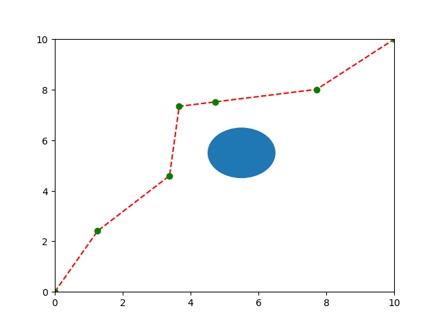
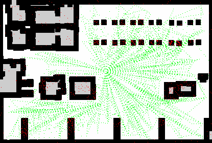
The following example shows a 2D point robot inside a 10x10 space with an ovular obstacle at position (5.5, 5.5):
from ompl import base as ob
from ompl import geometric as og
import math
from math import sqrt
import numpy as np
import matplotlib.pyplot as plt

# specify valid state condition
def isStateValid(state):
  x = state.getX()
  y = state.getY()
  if sqrt(pow(x - obstacle[0], 2) + pow(y - obstacle[1], 2)) - obstacle[2] <= 0:
    return False
  return True

def plan():
  # Construct the robot state space in which we're planning. We're
  # planning in [0,1]x[0,1], a subset of R^2.
  space = ob.SE2StateSpace()

  # set state space's lower and upper bounds
  bounds = ob.RealVectorBounds(2)
  bounds.setLow(0, dimensions[0])
  bounds.setLow(1, dimensions[1])
  bounds.setHigh(0, dimensions[2])
  bounds.setHigh(1, dimensions[3])
  space.setBounds(bounds)

  # construct a space information instance for this state space
  si = ob.SpaceInformation(space)
  # set state validity checking for this space
  si.setStateValidityChecker(ob.StateValidityCheckerFn(isStateValid))

  # Set our robot's starting and goal state
  start = ob.State(space)
  start().setX(0)
  start().setY(0)
  start().setYaw(math.pi / 4)
  goal = ob.State(space)
  goal().setX(10)
  goal().setY(10)
  goal().setYaw(math.pi / 4)

  # create a problem instance
  pdef = ob.ProblemDefinition(si)

  # set the start and goal states
  pdef.setStartAndGoalStates(start, goal)

  # create a planner for the defined space
  planner = og.RRTConnect(si)

  # set the problem we are trying to solve for the planner
  planner.setProblemDefinition(pdef)

  # perform setup steps for the planner
  planner.setup()

  # solve the problem and print the solution if exists
  solved = planner.solve(1.0)
  if solved:
    print(pdef.getSolutionPath())
    plot_path(pdef.getSolutionPath(), dimensions)

def create_numpy_path(states):
    lines = states.splitlines()
    length = len(lines) - 1
    array = np.zeros((length, 2))

    for i in range(length):
        array[i][0] = float(lines[i].split(" ")[0])
        array[i][1] = float(lines[i].split(" ")[1])
    return array

def plot_path(solution_path, dimensions):
  matrix = solution_path.printAsMatrix()
  path = create_numpy_path(matrix)
  x, y = path.T
  ax = plt.gca()
  ax.plot(x, y, 'r--')
  ax.plot(x, y, 'go')
  ax.axis(xmin=dimensions[0], xmax=dimensions[2], ymin=dimensions[1], ymax=dimensions[3])
  ax.add_patch(plt.Circle((obstacle[0], obstacle[1]), radius=obstacle[2]))

  plt.show()

if __name__ == "__main__":
  dimensions = [0, 0, 10, 10]
  obstacle = [5.5, 5.5, 1]   # [x, y, radius]
  plan()
Output:
Info:    RRTConnect: Space information setup was not yet called. Calling now.
Debug:   RRTConnect: Planner range detected to be 3.142586
Info:    RRTConnect: Starting planning with 1 states already in datastructure
Info:    RRTConnect: Created 9 states (4 start + 5 goal)
Geometric path with 7 states
Compound state [
RealVectorState [0 0]
SO2State [0.785398]
]
Compound state [
RealVectorState [1.26041 2.4087]
SO2State [-0.0626893]
]
Compound state [
RealVectorState [3.38076 4.59672]
SO2State [0.128782]
]
Compound state [
RealVectorState [3.66427 7.34115]
SO2State [0.895879]
]
Compound state [
RealVectorState [4.7318 7.51811]
SO2State [0.808152]
]
Compound state [
RealVectorState [7.7113 8.01201]
SO2State [0.563304]
]
Compound state [
RealVectorState [10 10]
SO2State [0.785398]
]
Plot:
To better understand how to use the library, it is highly recommended to go to the tutorials and demos sections of the official website.
Conversion From 3D to 2D
Robot Localization is the process of determining, where the robot is located regarding it’s environment. Localization is an important resource for us in solving this exercise. Localization can be accomplished in any way possible, be it Monte Carlo, Particle Filter, or even Offline Algorithms. Since we have a map available to us, offline localization is the best way to move forward. Offline Localization will involve converting from a 3D environment scan to a 2D map. There are again numerous ways to do it, but the technique used in exercise is using transformation matrices.
Transformation Matrices
In simple terms, transformation is an invertible function that maps a set X to itself. Geometrically, it moves a point to some other location in some space. Algebraically, all the transformations can be mapped using matrix representation. In order to apply transformation on a point, we multiply the point with the specific transformation matrix to get the new location. Some important transformations are:
- Translation
Translation of Euclidean Space(2D or 3D world) moves every point by a fixed distance in the same direction.
- Rotation
Rotation spins the object around a fixed point, known as center of rotation.
- Scaling
Scaling enlarges or diminishes objects, by a certain given scale factor.
- Shear
Shear rotates one axis so that the axes are no longer perpendicular.
In order to apply multiple transformations all at the same time, we use the concept of Transformation Matrix which enables us to multiply a single matrix for all the operations at once!
Transformation Matrix
In our case we need to map a 3D Point in gazebo, to a 2D matrix map of our house. The equation used in the exercise was:
Coordinate to Pixel Conversion Equation
In order to carry out the inverse operation of 3D to 2D, we can simply multiply, the pixel vector with the inverse of the transformation matrix to get the gazebo vector. The inverse of the matrix exists because the mapping is invertible and we do not care about the z coordinate of the environment, implying that each point in gazebo corresponds to a single point in the map.
Hints
Simple hints provided to help you solve the Amazon Warehouse exercise. Please note that the full solution has not been provided. Also, the hints are more related to the reference solution, since multiple solutions are possible for this exercise.
Ideas for solving the exercise
There are different ways to solve the exercise:
-
Euclidean planning
Define the robot as a 2D point and thicken the obstacles’ edges according to the robot’s radius to avoid collision, in this case, the state space can simply be an Euclidean space and all those black pixels will be invalid states. Maybe this demo can help you!
-
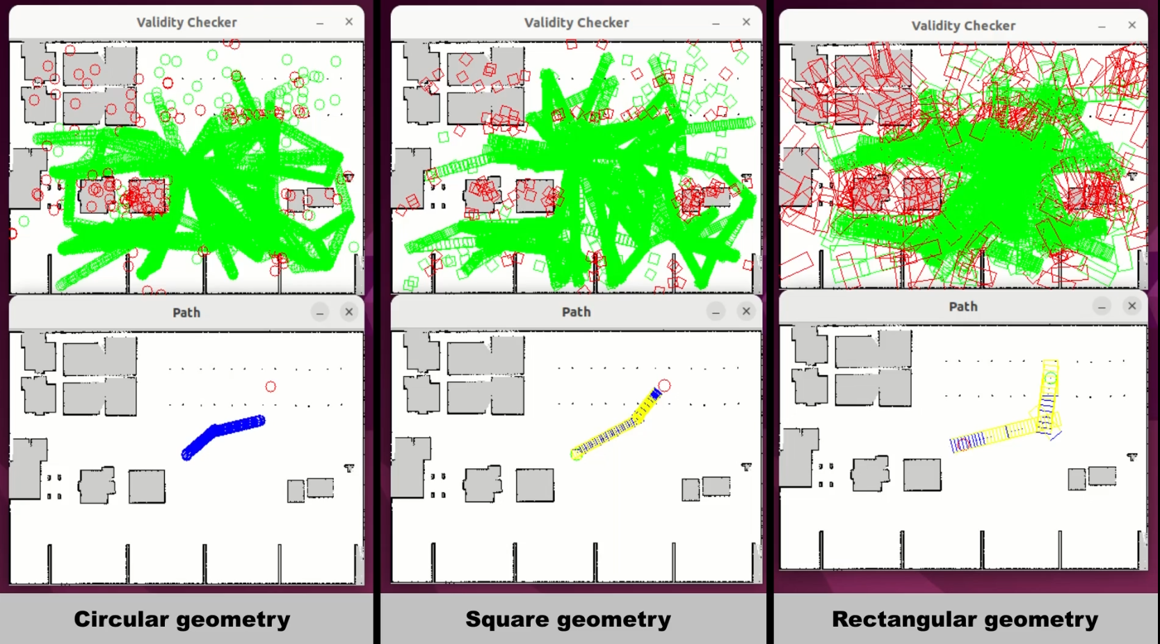
Planning with robot’s geometry constraints
Since the robot’s geometry is not always suitable to be approximated as a point, as in the case when the rectangular shelving is loaded, it would be a better way to solve the problem taking into consideration the robot’s geometry.
You can represent the robot as a set of pixels, so that a state will be valid when all pixels in the set are free. Now, it is no longer enough to use only Euclidean space but you must take into consideration the rotation of the robot. Therefore, it would be convenient to use a state space that includes that variable, such as SE2StateSpace. And what else? A motion validator will be also essential, to ensure the feasibility of transitioning between states.
You can make use of the DubinsStateSpace or ReedsSheppStateSpace to solve the exersice. Check this demo!
-
Control-based planning
In control-based planning, we need to define a control space and specify control propagation to set the robot movement constraints.
However, there is another approach using the OMPL app class. This class includes predefined robot types such as dynamic car, kinematic car, quadrotor, etc. And, we can define the state space using mesh files. Check this demo!
- For now, only the meshes of the Ackermann robot and Warehouse 1 are available (listed in the Supporting information section).
In this case, the solution path is composed of a sequence of controls (v, w, duration), instead of coordinates:
At state Compound state [
RealVectorState [0 0]
SO2State [0]
]
apply control RealVectorControl [3.76703 0.00946806]
for 1 steps
Besides, the Gazebo RTF factor can impact the accurary of plan execution, so using simulated time can lead to better results.
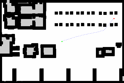
How to find the shortest path?
The library offers the possibility to set an optimization objective, which could be a great help in finding the shortest path. Check out in this tutorial how to do it!
Points to consider
- The loaded shelf is no longer a obstacle but part of the robot, then:
- the robot’s geometry changes.
- remember to exclude the shelf itself when defining invalid states.
Important points to remember
- Convert the coordinates from meter to pixel before representing with WebGUI.showPath(array).
Videos
Demonstrative video of completed solution
-
Euclidean planning
-
Planning with robot’s geometry constraints
-
Control-based planning
- Contributors: Lucía Lishan Chen Huang, Blanca Soria Rubio, Jose María Cañas
- Maintained by Lucía Lishan Chen Huang, Javier Izquierdo.