Localized Vacuum Cleaner
Goal
The objective of this exercise is to implement the logic of a navigation algorithm for an autonomous vacuum cleaner by making use of the location of the robot. The robot is equipped with a map and knows it’s current location in it. The main objective will be to cover the largest area of a house using the programmed algorithm.
Frequency API
import Frequency- to import the Frequency library class. This class contains the tick function to regulate the execution rate.Frequency.tick(ideal_rate)- regulates the execution rate to the number of Hz specified. Defaults to 50 Hz.
Robot API
import HAL- to import the HAL (Hardware Abstraction Layer) library class. This class contains the functions that send and receive information to and from the Hardware (Gazebo).-
import WebGUI- to import the WebGUI (Web Graphical User Interface) library class. This class contains the functions used to view the debugging information, like image widgets. HAL.setV()- to set the linear speed.-
HAL.setW()- to set the angular velocity. HAL.getPose3d().x- to get the X coordinate of the robot.HAL.getPose3d().y- to get the Y coordinate of the robot.HAL.getPose3d().yaw- to get the orientation of the robot.HAL.getBumperData().state- To establish if the robot has crashed or not. Returns a 1 if the robot collides and a 0 if it has not crashed.HAL.getBumperData().bumper- If the robot has crashed, it turns to 1 when the crash occurs at the center of the robot, 0 when it occurs at its right and 2 if the collision is at its left.HAL.getLaserData()- It allows to obtain the data of the laser sensor, which consists of 180 pairs of values (0-180º, distance in meters).WebGUI.showNumpy(mat)- Displays the matrix sent. Accepts an uint8 numpy matrix, values ranging from 0 to 127 for grayscale and values 128 to 134 for predetermined colors (128 = red; 129 = orange; 130 = yellow; 131 = green; 132 = blue; 133 = indigo; 134 = violet). Matrix should be square and the dimensions bigger than 100*100 for correct visualization. Dimensions bigger than 1000*1000 may affect performance.import numpy as np # Create a 400x400 matrix with random values between 0 and 127 (grayscale) matrix = np.random.randint(0, 128, (400, 400), dtype=np.uint8) # Add a red square region to the matrix x = np.random.randint(0, 391) y = np.random.randint(0, 391) matrix[x:x+10, y:y+10] = 128 WebGUI.showNumpy(matrix)WebGUI.getMap(url)- Returns a numpy array with the image data in a 3 dimensional array (R, G, B, A). The URL of the Vacuum Cleaner Loc map is ‘/resources/exercises/vacuum_cleaner_loc/mapgrannyannie.png’, so the instruction to get the map isarray = WebGUI.getMap('/resources/exercises/vacuum_cleaner_loc/images/mapgrannyannie.png')
For this example, it is necessary to ensure that the vacuum cleaner covers the highest possible percentage of the house. The application of the automatic evaluator (referee) will measure the percentage traveled, and based on this percentage, will perform the qualification of the solution algorithm.
Types conversion
Laser
import math
import numpy as np

def parse_laser_data(laser_data):
    """ Parses the LaserData object and returns a tuple with two lists:
        1. List of polar coordinates, with (distance, angle) tuples,
           where the angle is zero at the front of the robot and increases to the left.
        2. List of cartesian (x, y) coordinates, following the ref. system noted below.

        Note: The list of laser values MUST NOT BE EMPTY.
    """
    laser_polar = []  # Laser data in polar coordinates (dist, angle)
    laser_xy = []  # Laser data in cartesian coordinates (x, y)
    for i in range(180):
        # i contains the index of the laser ray, which starts at the robot's right
        # The laser has a resolution of 1 ray / degree
        #
        #                (i=90)
        #                 ^
        #                 |x
        #             y   |
        # (i=180)    <----R      (i=0)

        # Extract the distance at index i
        dist = laser_data.values[i]
        # The final angle is centered (zeroed) at the front of the robot.
        angle = math.radians(i - 90)
        laser_polar += [(dist, angle)]
        # Compute x, y coordinates from distance and angle
        x = dist * math.cos(angle)
        y = dist * math.sin(angle)
        laser_xy += [(x, y)]
    return laser_polar, laser_xy

# Usage
laser_data = HAL.getLaserData()
if len(laser_data.values) > 0:
    laser_polar, laser_xy = parse_laser_data(laser_data)
Videos
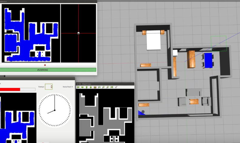
This solution is an illustration for the Web Templates
Theory
As the problem may have multiple solutions, only the theory behind the reference solution has been covered.
Conversion From 3D to 2D
Robot Localization is the process of determining, where the robot is located regarding it’s environment. Localization is an important resource to us in solving this exercise. Localization can be accomplished in any way possible, be it Monte Carlo, Particle Filter, or even Offline Algorithms. Since we have a map available to us, offline localization is the best way to move forward. Offline Localization will involve converting from a 3D environment scan to a 2D map. There are again numerous ways to do it, but the technique used in exercise is using transformation matrices.
Transformation Matrices
In simple terms, transformation is an invertible function that maps a set X to itself. Geometrically, it moves a point to some other location in some space. Algebraically, all the transformations can be mapped using matrix representation. In order to apply transformation on a point, we multiply the point with the specific transformation matrix to get the new location. Some important transformations are:
- Translation
Translation of Euclidean Space(2D or 3D world) moves every point by a fixed distance in the same direction.
- Rotation
Rotation spins the object around a fixed point, known as center of rotation.
- Scaling
Scaling enlarges or diminishes objects, by a certain given scale factor.
- Shear
Shear rotates one axis so that the axes are no longer perpendicular.
In order to apply multiple transformations all at the same time, we use the concept of Transformation Matrix which enables us to multiply a single matrix for all the operations at once!
Transformation Matrix
In our case we need to map a 3D Point in gazebo, to a 2D matrix map of our house. The equation used in the exercise was:
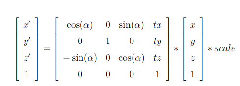
Coordinate to Pixel Conversion Equation
In order to carry out the inverse operation of 3D to 2D, we can simply multiply the pixel vector by the inverse of the transformation matrix to get the gazebo vector. The inverse of the matrix exists because the mapping is invertible and we do not care about the z coordinate of the environment, implying that each point in gazebo corresponds to a single point in the map.
Coverage and Decomposition
After the robot is localized in it’s environment, we can employ decomposition techniques in our algorithm, to deal with the actual coverage of the surroundings. There are lot of decomposition techniques available for our use. The Decomposition Algorithm, decomposes the map into separate segments, which our robot can cover one by one. Decomposition can be directly related to Graph Theory, where the segments are taken as nodes and the edges connecting nodes depict that the adjacent segments share a common boundary. The robot can path plan to the nearest node and then start sweeping again! Most of the details regarding decomposition would be implementation.
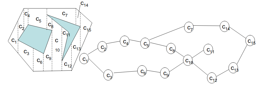
Adjacency Graph
Travelling between segments
Once a certain segment has been swept. In order to reach the next segment (preferably nearest one) there are again a multitude of path planning algorithms. The algorithm used in the reference solution is the Visibility Algorithm. As the name suggests, visibility of the target is the basic building block. So, let’s define visibility first off all!
If a straight line exists between two points, and the line does not pass over obstacles, the two points are said to be visible to each other. Mathematically speaking, the two points under consideration must satisfy a common equation.
Equation of a Line
Starting from the destination cell, the robot can map it’s path one cell at a time, while keeping visibility as a reference, until it reaches the current cell, the robot is present in. Once, the plan has been decided the robot can follow that path and reach it’s destination.
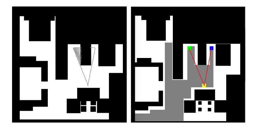
Visibility Error
But, sometimes due to close proximity to corner, the robot may collide with it. To avoid the occurrence of any such event, we may also consider dilation techniques, since the map used is a binary image. Erosion is a Morphology Function that erodes away the boundaries of foreground object (white is the object in foreground). Refer to this link for more information on erosion.
Morphological Operations
Hints
Simple hints provided to help you solve the vacuum_cleaner_loc exercise. Please note that the full solution has not been provided. Also, the hints are more related to the reference solution, since multiple solutions are possible for this exercise.
Grid Representation
Due to the involvement of Localization in this exercise, we are given a map of the surroundings of the robot, which it needs to cover. The map is present in the directory path resources/images/. But since we are using path planning and decomposition algorithms. These are very easy to implement on a grid like structure. Although any data structure, representing adjacency graph would suffice. See the illustrations for what happens without using any data structure(a brute force approach). To implement grids on images, we need to apply basic image processing, which can be accomplished easily using the opencv library.
The first step would be to apply erosion function on the map image. This is done in order to ensure some degree of distance between our robot and obstacle during runtime.
The second task is to come up with a transformation matrix, that would convert our 3d gazebo positions into 2d map representations. A degree of rotation has to applied on the Y axis and add a translation of 0.6 on the X axis and -1 on the Y axis can be used to get the origin of coordinates (0, 0) of the image in the upper left hand corner.
Once we get specific positions on our map. Using the dimensions of our vacuum cleaner, we can generate grid cells around those points. The size of vacuum cleaner can be taken as 35x35 pixel units. Take it as an exercise to calculate it on your own!
Obstacles and Color Coding
Taking the map as a grayscale image, we can apply color coding to the map as well. It is convenient to separate Obstacles, Virtual Obstacles, Return Points and Critical Points
In the context of this exercise,
- Obstacles: The obstacles in our map that our robot cannot go over.
- Virtual Obstacles: The grid cell that our robot has covered.
- Return Points: Starting points of the decomposed cells.
- Critical Points: The points where our robot has stuck between obstacles and virtual obstacles. It is from critical points, that our robot has to start moving towards the next return point.
Checking for Points
Defining different points simplifies the algorithm as well!
-
Return Points Return Points can be checked while the robot is in zig-zag motion. Empty cells near the robot can be classified as return points. The list of Return Points has to be kept dynamic in order to insert and pop the points whenever required.
-
Critical Points Critical Points can be classified whenever our robot is stuck around Obstacles or Virtual Obstacles and cannot move any further.
-
Checking for Arrival of Cell Considering various offset errors in the real world(consider simulation to be real world as well!). Arrival of the robot in a particular cell should be considered within a margin of error, otherwise the robot may start oscillating, in the search of a cell on which it can never arrive.
-
Efficient Turning and Straight Motion One trick to adjust the speed and direction of motion is to keep the next 3 cells of the robot which are in it’s direction of motion under consideration.
- All 3 cells are free Make the robot move at maximum speed
- 2 cells are free Make the robot move at a fast speed
- 1 cell is free Along with small linear motion forward, start applying rotation as well
- 0 cells are free Stop the robot and apply only rotation
As a final note, quite a lot of tips and tricks regarding implementation have been discussed in this page. This is a tough exercise, which may take quite a lot of time to solve. The main objective of the exercise is to cover a significant area of the house, without taking time into consideration.
Illustrations
Grid Based Approach

PID Based(without grid) Approach
Demonstrative video of the solution
Contributors
- Contributors: Vanessa Fernandez, Jose María Cañas, Carlos Awadallah, Nacho Arranz, Javier Izquierdo.
- Maintained by Sakshay Mahna, Javier Izquierdo.
References
The major credit for this coverage algorithm goes to Jose María Cañas and his student Irene Lope.
- https://onlinelibrary.wiley.com/doi/full/10.1002/047134608X.W8318
- https://en.wikipedia.org/wiki/Transformation_(function)
- https://www.cs.cmu.edu/~motionplanning/lecture/Chap6-CellDecomp_howie.pdf
- http://correll.cs.colorado.edu/?p=965
- https://homepages.inf.ed.ac.uk/rbf/HIPR2/dilate.htm
- https://gsyc.urjc.es/jmplaza/students/tfg-Robotics_Academy-irene_lope-2018.pdf
One of the best video series on Linear Algebra