Basic Vacuum Cleaner
Goal
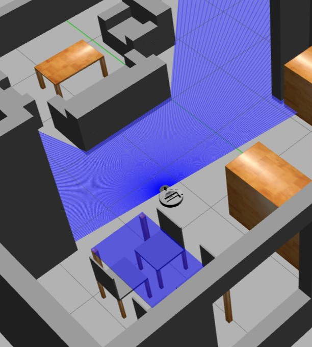
The objective of this practice is to implement the logic of a navigation algorithm for an autonomous vacuum. The main objective will be to cover the largest area of a house using the programmed algorithm.
For this example, it is necessary to ensure that the vacuum cleaner covers the highest possible percentage of the house. The application of the automatic evaluator (in Unibotics) will measure the percentage traveled, and based on this percentage, will perform the qualification of the solution algorithm.
Frequency API
Python
import Frequency- to import the Frequency library class. This class contains the tick function to regulate the execution rate.Frequency.tick(ideal_rate)- regulates the execution rate to the number of Hz specified. Defaults to 50 Hz.
C++
#include "Frequency.hpp"- to import the Frequency library class. This class contains the tick function to regulate the execution rate.Frequency freq = Frequency();- to instanciate the Frequency class.freq.tick(ideal_rate);- regulates the execution rate to the number of Hz specified. Defaults to 50 Hz.
Robot API
This exercise now supports ROS 2-direct implementation in addition to the original HAL-based approach. Below you’ll find the details for both options.
HAL-based Implementation
Python
import HAL- to import the HAL (Hardware Abstraction Layer) library class. This class contains the functions that send and receive information to and from the Hardware (Gazebo).import WebGUI- to import the WebGUI (Web Graphical User Interface) library class. This class contains the functions used to view the debugging information, like image widgets.HAL.getBumperData().state- to establish if the robot has crashed or not. Returns 1 if the robot collides and 0 if it has not crashed. DISABLED: use laser data in the center (90) to get the same result.HAL.getBumperData().bumper- if the robot has crashed, it returns 1 when the crash occurs on center of the robot, 0 when it occurs on its right and 2 if the collision is on its left. DISABLED: use laser data in the center (90) to get the same result.HAL.setV()- to set the linear speed.HAL.setW()- to set the angular velocity.HAL.getLaserData()- It allows to obtain the data of the laser sensor, which consists of 180 pairs of values (0-180º, distance in meters).
Here is an example of how to parse the laser data:
import math
import numpy as np

def parse_laser_data(laser_data):
    """ Parses the LaserData object and returns a tuple with two lists:
        1. List of  polar coordinates, with (distance, angle) tuples,
           where the angle is zero at the front of the robot and increases to the left.
        2. List of cartesian (x, y) coordinates, following the ref. system noted below.

        Note: The list of laser values MUST NOT BE EMPTY.
    """
    laser_polar = []  # Laser data in polar coordinates (dist, angle)
    laser_xy = []  # Laser data in cartesian coordinates (x, y)
    for i in range(180):
        # i contains the index of the laser ray, which starts at the robot's right
        # The laser has a resolution of 1 ray / degree
        #
        #                (i=90)
        #                 ^
        #                 |x
        #             y   |
        # (i=180)    <----R      (i=0)

        # Extract the distance at index i
        dist = laser_data.values[i]
        # The final angle is centered (zeroed) at the front of the robot.
        angle = math.radians(i - 90)
        laser_polar += [(dist, angle)]
        # Compute x, y coordinates from distance and angle
        x = dist * math.cos(angle)
        y = dist * math.sin(angle)
        laser_xy += [(x, y)]
    return laser_polar, laser_xy

# Usage
laser_data = HAL.getLaserData()
if len(laser_data.values) > 0:
    laser_polar, laser_xy = parse_laser_data(laser_data)
C++
#include "HAL.hpp"- to import the HAL (Hardware Abstraction Layer) library class. This class contains the functions that send and receive information to and from the Hardware (Gazebo).#include "WebGUI.hpp"- to import the WebGUI (Web Graphical User Interface) library class. This class contains the functions used to view the debugging information, like image widgets.HAL::get_laser_data();- It allows to obtain the data of the laser sensor (LaserData), which consists of 180 pairs of values (0-180º, distance in meters).HAL::set_v(velocity);- to set the linear speed.HAL::set_w(velocity);- to set the angular velocity.HAL::get_bumper_data();- to get the bumper state from the robot. Returns a vector of booleans with the next order: Right, Center, Left. DISABLED: use laser data in the center (90) to get the same result.
In order to use the HAL-based controls you must include the following lines:
#include "HAL.hpp"
#include "WebGUI.hpp"
#include "Frequency.hpp"

void exercise() {
    Frequency freq = Frequency();
    // Enter sequential code!

    while (true)
    {
        // Enter iterative code!
        freq.tick();


    }
}
ROS 2-direct Implementation
Use standard ROS 2 topics for direct communication with the simulation.
/cmd_vel- Publish to this topic to set both linear and angular velocities. Message type:geometry_msgs/msg/Twist/roombaROS/laser/scan- Subscribe to this topic to get laser scan data. Message type:sensor_msgs/msg/LaserScan/roombaROS/events/center_bumper- Subscribe to this topic to detect collisions at the center of the robot. Message type:gazebo_msgs/msg/ContactsState.DISABLED: use laser data in the center (90) to get the same result./roombaROS/events/left_bumper- Subscribe to this topic to detect collisions at the left side of the robot. Message type:gazebo_msgs/msg/ContactsState. DISABLED: use laser data in the center (90) to get the same result./roombaROS/events/right_bumper- Subscribe to this topic to detect collisions at the right side of the robot. Message type:gazebo_msgs/msg/ContactsState. DISABLED: use laser data in the center (90) to get the same result.
Python
Note: Ensure this import is included in your script to access the Web GUI functionalities.
import WebGUI - to enable the Web GUI for visualizing camera images.
To have frequency control you need to use standard ROS 2 mechanisms to manage loop timing:
rclpy.spin()- Event-driven execution using callbacks.rclpy.spin_once()- Single-step processing, often with custom timers.rclpy.Rate()- Loop-based frequency control.
Note
WebGUI already initializes rclpy internally, so this should be taken into account when building a direct ROS 2 solution.
C++
In order to use direct ros controls you must include the following lines:
#ifndef USER_NODE
#define USER_NODE

#include "rclcpp/rclcpp.hpp"

class UserNode : public rclcpp::Node {
  // Your class
};

#endif
You must define USER_NODE and a UserNode node class.
To have frequency control you may use a timer and a control function as follows:
  UserNode() : Node("user_node")
  {
    // More subscribers and publishers
    timer_ = create_wall_timer(100ms, std::bind(&UserNode::control_cycle, this));
  };

// More Code

  void control_cycle(){
    // Your function
  };
Theory
Implementation of navigation algorithms for an autonomous vacuum is the basic requirement for this exercise. The main objective is to cover the largest area of a house. First, let us understand what are Coverage Algorithms.
Coverage Algorithms
Coverage Path Planning is an important area of research in Path Planning for robotics, which involves finding a path that passes through every reachable position in its environment. In this exercise, We are using a very basic coverage algorithm called Random Exploration.
Analyzing Coverage Algorithms
Classification
Coverage algorithms are divided into two categories.
-
Offline coverage Uses fixed information and the environment is known in advance. Genetic Algorithms, Neural Networks, Cellular Decomposition, Spanning Trees are some examples to name a few.
-
Online Coverage
Uses real-time measurements and decisions to cover the entire area. The Sensor-based approach is included in this category.
Base Movement
The problem of coverage involves two standard basic motions, which are used as a base for other complex coverage algorithms.
- Spiral Motion
The robot follows an increasing circle/square pattern.

- Boustrophedon Motion
The robot follows an S-shaped pattern.

Analysis of Coverage Algorithms
Any coverage algorithm is analyzed using the given criterion.
-
Environment Decomposition This involves dividing the area into smaller parts.
-
Sweep Direction
This influences the optimality of generated paths for each sub-region by adjusting the duration, speed, and direction of each sweep.
- Optimal Backtracking
This involves the plan to move from one small subregion to another. The coverage is said to be complete when there is no point left to backtrack.
Supplements
Usually, coverage algorithms generate a linear, piecewise path composed of straight lines and sharp turns. This path is difficult to follow for other autonomous drones like Underwater Vehicles, Aerial Vehicles and some Ground Vehicles. Path Smoothening is applied to these paths to effectively implement the algorithm.
Hints
Simple hints provided to help you solve the vacuum_cleaner exercise. Please note that the full solution has not been provided.
Random Angle Generation
The most important task is the generation of a random angle. There are 2 ways to achieve it.
-
Random Duration: By keeping the angular_velocity fixed, the duration of the turn can be randomized, in order to point the robot towards a random direction.
-
Random Angle: This method requires calculation. We generate a random angle and then turn towards it. Approximately an angular speed of 3 turns the robot by 90 degrees.
Among both methods, Random Duration would be preferable as the Random Angle requires precision, which requires PID to be achieved successfully.
Also, in order to achieve better precision it is preferable to use rospy.sleep() in place of time.sleep().
Dash Movement
Once the direction has been decided, we move in that direction. This is the simplest part, we have to send a velocity changing command to the robot, and wait until a collision is detected.
A word of caution though, whenever we have a change of state, we have to give a sleep duration to the robot to give it time to reset the commands given to it. Illustrations section describes a visual representation.
Spiral Movement
Using the physical formula $v = r·\omega$ (See references for more details). In order to increase $r$, we can either increase $v$ or decrease $\omega$, while keeping the other parameter constant. Experimentally, increasing $v$ has a better effect than decreasing $\omega$. Refer to illustrations.
Analysis
Being such a simple algorithm, it is not expected to work all the time. The maximum accuracy we got was 80% and that too only once!
Illustrations
Without applying a sleep duration the previous rotation command still has effect on the go straight command
After applying a duration, we get straight direction movement
Effect of reducing $\omega$ to generate spiral
Effect of increasing $v$ to generate spiral
Demonstrative video of the solution
Contributors
- Contributors: Vanessa Fernandez, Jose María Cañas, Carlos Awadallah, Nacho Arranz, Javier Izquierdo, Ashish Ramesh.
- Maintained by Javier Izquierdo.