Laser Mapping
Goal
The goal of this exercise is to develop a navigation algorithm that allows a robot to autonomously explore a warehouse environment while generating an accurate 2D map of the surroundings using LIDAR sensor data.
The robot must be able to:
- Perceive obstacles and free space using laser measurements
- Build and update a map of the environment while moving
- Navigate safely without prior knowledge of the environment
- Continue exploration until the reachable area is sufficiently covered
Frequency API
Python
import Frequency- to import the Frequency library class. This class contains the tick function to regulate the execution rate.Frequency.tick(ideal_rate)- regulates the execution rate to the number of Hz specified. Defaults to 50 Hz.
C++
#include "Frequency.hpp"- to import the Frequency library class. This class contains the tick function to regulate the execution rate.Frequency freq = Frequency();- to instanciate the Frequency class.freq.tick(ideal_rate);- regulates the execution rate to the number of Hz specified. Defaults to 50 Hz.
Available Worlds
This exercise has six universes divided into two environments, each with three odometry noise levels. The selected universe determines how much drift accumulates in the robot’s odometry over time.
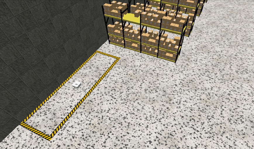
Small Warehouse — compact environment, recommended for getting started:
- Small Laser Mapping Warehouse — low odometry noise.
- Small Laser Mapping Warehouse Medium Noise — medium odometry noise.
- Small Laser Mapping Warehouse High Noise — high odometry noise.
Large Warehouse — larger and more complex environment:
- Laser Mapping Warehouse Low Noise — low odometry noise.
- Laser Mapping Warehouse Medium Noise — medium odometry noise.
- Laser Mapping Warehouse High Noise — high odometry noise.
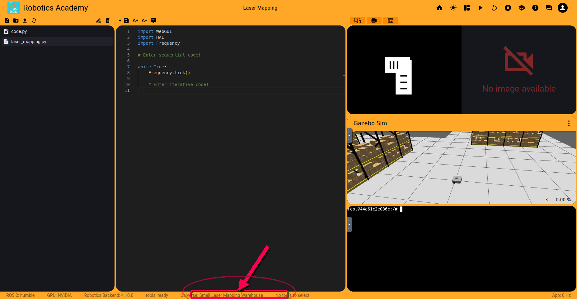
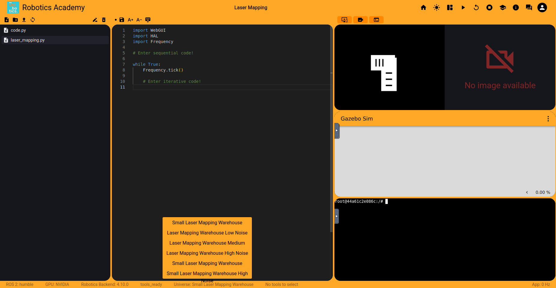
To select a universe, click on the universe name in the bottom toolbar and pick the desired world from the dropdown.
The robot provides two sources of position information:
HAL.getPose3d().x,HAL.getPose3d().y,HAL.getPose3d().yaw— absolute position of the robot.HAL.getOdom().x,HAL.getOdom().y,HAL.getOdom().yaw— noisy odometry. The noise level depends on the selected universe.
Robot API
This exercise now supports ROS 2-native implementation in addition to the original HAL-based approach. Below you’ll find the details for both options.
HAL-based Implementation
Python
import HAL- to import the HAL library class. This class contains the functions that receive information from the sensors or work with the actuators.import WebGUI- to import the WebGUI (Web Graphical User Interface) library class. This class contains the functions used to view the debugging information, like image widgets.HAL.getPose3d().x- to get position x of the robot.HAL.getPose3d().y- to get position y of the robot.HAL.getPose3d().yaw- to get the orientation of the robot.HAL.getOdom().x- to get the approximated X coordinate of the robot (with noise). The noise level depends on the selected world.HAL.getOdom().y- to get the approximated Y coordinate of the robot (with noise). The noise level depends on the selected world.HAL.getOdom().yaw- to get the approximated orientation of the robot (with noise). The noise level depends on the selected world.HAL.setW()- to set the angular velocity.HAL.setV()- to set the linear velocity.HAL.getLaserData()- to get the data of the LIDAR. Which consists of 360 values.WebGUI.poseToMap(x, y, yaw)- converts a gazebo world coordinate system position to a map pixel.WebGUI.setUserMap(map)- shows the user built map on the user interface. It represents the values of the field that have been assigned to the array passed as a parameter. Accepts as input a two-dimensional uint8 numpy array whose values can range from 0 to 255 (grayscale). The array must be 970 pixels high and 1500 pixels wide.
C++
#include "HAL.hpp"- to import the HAL (Hardware Abstraction Layer) library class. This class contains the functions that send and receive information to and from the Hardware (Gazebo).#include "WebGUI.hpp"- to import the WebGUI (Web Graphical User Interface) library class. This class contains the functions used to view the debugging information, like image widgets.HAL::set_v(velocity);- sets the linear velocity of the robot. The input is afloat. Returnsvoid.HAL::set_w(velocity);- sets the angular velocity of the robot. The input is afloat. Returnsvoid.HAL::get_pose3d();- returns the current ground-truth robot pose as aHAL::Pose3d.HAL::get_pose3d().x;- gets the robot x position in world coordinates (double).HAL::get_pose3d().y;- gets the robot y position in world coordinates (double).HAL::get_pose3d().yaw;- gets the robot orientation around the vertical axis in world coordinates (double).HAL::get_odom();- returns the noisy odometry pose as aHAL::Pose3d. The noise level depends on the selected world.HAL::get_odom().x;- gets the noisy odometry x position (double).HAL::get_odom().y;- gets the noisy odometry y position (double).HAL::get_odom().yaw;- gets the noisy odometry orientation around the vertical axis (double).HAL::get_laser_data();- returns the laser sensor data as aHAL::LaserData.HAL::get_laser_data().values;- contains the laser distance readings as astd::vector<float>.HAL::get_laser_data().minAngle;- minimum laser angle (double).HAL::get_laser_data().maxAngle;- maximum laser angle (double).HAL::get_laser_data().minRange;- minimum valid laser range (double).HAL::get_laser_data().maxRange;- maximum valid laser range (double).WebGUI::pose_to_map(x, y, yaw);- converts a robot pose from Gazebo world coordinates to map pixel coordinates. The inputs aredoublevalues. Returns astd::vector<double>.WebGUI::set_user_map(image);- displays the user-built occupancy map in the WebGUI. The input must be acv::Mat. Returnsvoid.
In order to use the HAL-based controls you must include the following lines:
#include "HAL.hpp"
#include "WebGUI.hpp"
#include "Frequency.hpp"

void exercise() {
    Frequency freq = Frequency();
    // Enter sequential code!

    while (true)
    {
        // Enter iterative code!
        freq.tick();


    }
}
C++ API examples
-
Example to get the robot pose:
HAL::Pose3d odom = HAL::get_odom(); double odom_x = odom.x; double odom_y = odom.y; double odom_yaw = odom.yaw; -
Example to get laser data:
HAL::LaserData laser = HAL::get_laser_data(); if (!laser.values.empty()) { float first_distance = laser.values[0]; } -
Example to convert a robot pose to map coordinates:
std::vector<double> map_pose = WebGUI::pose_to_map(robot_x, robot_y, robot_yaw); double map_x = map_pose[0]; double map_y = map_pose[1]; double map_yaw = map_pose[2]; -
Example to show the generated occupancy map:
cv::Mat user_map(970, 1500, CV_8UC1, cv::Scalar(127));

WebGUI::set_user_map(user_map);
ROS 2-direct Implementation
Use standard ROS 2 topics for direct communication with the simulation.
-
/do150/cmd_vel- Publish to this topic to set both linear and angular velocities. Message type:geometry_msgs/msg/Twist -
/do150/odom- Subscribe to this topic to receive the robot ground-truth odometry. Message type:nav_msgs/msg/Odometry -
/do150/odom_noisy- Subscribe to this topic to receive the noisy odometry. Message type:nav_msgs/msg/Odometry -
/do150/laser/scan- Subscribe to this topic to receive laser data. Message type:sensor_msgs/msg/LaserScan
For image debugging:
/webgui/user_map- Publish to this topic to display the generated occupancy map in the WebGUI. Message type:sensor_msgs/msg/Image
QoS:TRANSIENT_LOCAL, depth1The map sent to/webgui/user_mapmust be amono8image with 1500 pixels width and 970 pixels height.
Python
Note: Ensure this import is included in your script to access the Web GUI functionalities.
import WebGUI - to enable the Web GUI for visualizing camera images.
To have frequency control you need to use standard ROS 2 mechanisms to manage loop timing:
rclpy.spin()- Event-driven execution using callbacks.rclpy.spin_once()- Single-step processing, often with custom timers.rclpy.Rate()- Loop-based frequency control.
Note
WebGUI already initializes rclpy internally, so this should be taken into account when building a direct ROS 2 solution.
C++
In order to use direct ros controls you must include the following lines:
#ifndef USER_NODE
#define USER_NODE

#include "rclcpp/rclcpp.hpp"

class UserNode : public rclcpp::Node {
  // Your class
};

#endif
You must define USER_NODE and a UserNode node class.
To have frequency control you may use a timer and a control function as follows:
  UserNode() : Node("user_node")
  {
    // More subscribers and publishers
    timer_ = create_wall_timer(100ms, std::bind(&UserNode::control_cycle, this));
  };

// More Code

  void control_cycle(){
    // Your function
  };
Theory
Laser mapping is the process by which a robot builds a representation of an unknown environment using distance measurements obtained from a LIDAR sensor while moving through the space. The robot continuously senses its surroundings, updates the map, and decides where to move next in order to reduce unexplored areas.
Mapping with known possitions
The robot uses its current position and orientation to correctly place sensor measurements into a global map. Each laser beam is described by a distance and an angle relative to the robot, which are converted into Cartesian coordinates. These points are then projected onto a grid map representing the environment. By repeating this process over time, the robot consistently marks free space and obstacles in the correct locations, gradually building an accurate map of its surroundings.
Analyzing Coverage Algorithms
Mapping with known positions assumes that the current position of the robot is known. This technique consists of converting the distance measurements of the different laser beams into Cartesian coordinates relative to the robot. The distance mesured by the beam can reflect the existence of an obstacle; therefore, these Cartesian coordinates are inserted reflecting obstacles in an occupation grid relative to the current position of the robot. This technique is not entirely real because in most cases, the position of the robot is unknown. Therefore, other techniques such as SLAM are used in real life.
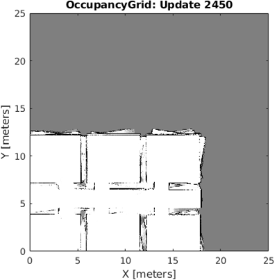
Occupancy grid
An occupation grid is a discretization of the robot’s environment in cells. This discretization will be given by the size of the world in which the robot is located. Each cell can represent free space, an obstacle, or an unexplored area. Instead of using fixed binary values, the belief of a cell is updated probabilistically using laser sensor measurements. When a laser beam passes through a cell, the confidence that the cell is free increases. When a laser beam ends at a cell, the confidence that the cell is occupied increases.
To combine observations over time in a stable way, the grid is updated using a log-odds representation. In this representation, probabilities are stored in a logarithmic form, allowing evidence from multiple measurements to be added incrementally. Positive log-odds values indicate a higher confidence of an obstacle, negative values indicate free space, and values close to zero correspond to unknown areas.
Laser Ray Interpretation and Measurement Independence
A single laser measurement provides information about both free space and obstacles. The space between the robot and the detected point is considered free, while the point where the laser ends represents an obstacle. Only the region up to the detected obstacle is interpreted, so areas behind walls are not incorrectly marked.
For probabilistic mapping to remain consistent, laser measurements should be treated as independent observations. Since repeated scans taken without sufficient movement are highly correlated, updates are considered meaningful only after the robot has moved or changed its orientation. This helps prevent overconfidence and improves the overall quality of the map.
Exploration and Coverage
Exploration defines the path that the robot follows to observe and map unknown areas of the environment. Different exploration algorithms generate different robot paths.
- Random Exploration-The robot moves along irregular paths, changing direction when obstacles are encountered.
- Wall-Following Exploration-The robot follows paths that remain close to walls or obstacles, allowing it to trace boundaries and gradually reveal the structure of the environment.
- Systematic Coverage (Lawn-Mower Motion)-The robot follows parallel back-and-forth paths that sweep the environment in an organized manner, ensuring uniform and predictable coverage.
- Frontier-Based Exploration-The robot’s path is directed toward the boundary between explored and unexplored regions, causing the mapped area to expand outward until no unknown space remains.
Any exploration algorithm that guides the robot safely through the environment and progressively reduces unknown areas is considered valid for this exercise.
Illustrations
Videos
This is a demostrative solution on unibotics.org
This solution is an illustration for the Web Templates
Contributors
- Contributors: Vladislav, Jose María Cañas, Nacho Arranz.
- Maintained by Juan Manuel Carretero.