MonteCarlo laser-based robot localization

Goal

The aim of this practical is to develop a localisation algorithm based on the particle filter using the robot’s laser.

Montecarlo Laser Loc — MonteCarlo Laser Location.

Instructions

This is the preferred way for running the exercise.

Installation

Clone the Robotics Academy repository on your local machine

git clone https://github.com/JdeRobot/RoboticsAcademy

Download Docker. Windows users should choose WSL 2 backend Docker installation if possible, as it has better performance than Hyper-V.
Pull the current distribution of Robotics Academy Docker Image

docker pull jderobot/robotics-academy:latest

How to perform the exercise?

Start a new docker container of the image and keep it running in the background.

docker run --rm -it -p 7164:7164 -p 2303:2303 -p 1905:1905 -p 8765:8765 -p 6080:6080 -p 1108:1108 jderobot/robotics-academy 

On the local machine navigate to 127.0.0.1:7164/ in the browser and choose the desired exercise.
Wait for the Connect button to turn green and display “Connected”. Click on the “Launch” button and wait for some time until an alert appears with the message Connection Established and button displays “Ready”.
The exercise can be used after the alert.

Where to insert the code?

In the launched webpage, type your code in the text editor,

from GUI import GUI
from HAL import HAL
# Enter sequential code!


while True:
    # Enter iterative code!

Using the Interface

Control Buttons: The control buttons enable the control of the interface. Play button sends the code written by User to the Image. Stop button stops the code that is currently running on the Image. Save button saves the code on the local machine. Load button loads the code from the local machine. Reset button resets the simulation (primarily, the image of the camera).
Brain and GUI Frequency: This input shows the running frequency of the iterative part of the code (under the while True:). A smaller value implies the code runs less number of times. A higher value implies the code runs a large number of times. The numerator is the one set as the Measured Frequency who is the one measured by the computer (a frequency of execution the computer is able to maintain despite the commanded one) and the input (denominator) is the Target Frequency which is the desired frequency by the student. The student should adjust the Target Frequency according to the Measured Frequency.
RTF (Real Time Factor): The RTF defines how much real time passes with each step of simulation time. A RTF of 1 implies that simulation time is passing at the same speed as real time. The lower the value the slower the simulation will run, which will vary depending on the computer.
Pseudo Console: This shows the error messages related to the student’s code that is sent. In order to print certain debugging information on this console. The student is provided with console.print() similar to print() command in the Python Interpreter.

Robot API

from HAL import HAL - to import the HAL library class. This class contains the functions that receives information from the webcam.
from GUI import GUI - to import the GUI (Graphical User Interface) library class. This class contains the functions used to view the debugging information, like image widgets.
HAL.getPose3d().x - to get position x of the robot
HAL.getPose3d().y - to get position y of the robot
HAL.getPose3d().yaw - to get the orientation of the robot
HAL.motors.sendW() - to set the angular velocity
HAL.motors.sendV() - to set the linear velocity
HAL.getLaserData() - to get the data of the LIDAR
HAL.getSonarData_0() - to get the sonar data of the sonar 1
HAL.getSonarData_1() - to get the sonar data of the sonar 2
HAL.getSonarData_2() - to get the sonar data of the sonar 3
HAL.getSonarData_3() - to get the sonar data of the sonar 4
HAL.getSonarData_4() - to get the sonar data of the sonar 5
HAL.getSonarData_5() - to get the sonar data of the sonar 6
HAL.getSonarData_6() - to get the sonar data of the sonar 7
HAL.getSonarData_7() - to get the sonar data of the sonar 8
GUI.showParticles(particles) - shows the particles on the map. It is necessary to pass a list of particles as an argument. Each particle must be a list with [positionx, positiony, angle].
GUI.showPose3D(pose) - shows the estimated position in the 3D viewer. It is necessary to pass a list with [positionx, positiony, positionz]. The 3D viewer will also show the real position of the robot, so you can compare how good your algorithm is.

Theory

Probabilistic localisation seeks to estimate the position of the robot and the model of the surrounding environment:

A. Probabilistic motion model. Due to various sources of noise (bumps, friction, imperfections of the robot, etc.) it is very difficult to predict the movement of the robot accurately. Therefore, it would be more convenient to describe this movement by means of a probability function, which will move with the robot’s movements [1].
B. Probabilistic model of sensory observation. It is related to the sensor measurements at each instant of time. This model is built by taking observations at known positions in the environment and calculating the probability that the robot is in each of these positions [2].
C. Probability fusion. This consists of accumulating the information obtained at each time instant, something that can be done using Bayes’ theorem. This fusion achieves that in each observation some modes of the probability function go up and others go down, so that as the number of iterations advances, the probability will be concentrated in only one of the modes, which will indicate the position of the robot [3].

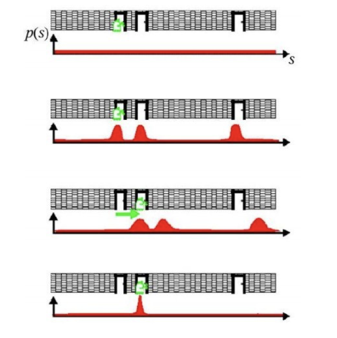
The following figure shows an example of probabilistic localisation. In the first phase, the robot does not know its initial state, the initial probability distribution is uniform. In the second phase, the robot is looking at a door, the sensory observation model determines that there are three zones or modes with equal probability of being the zone where the robot is. In the third phase, the robot is moving forward so the probabilistic motion model is applied, the probability distribution should move the same distance that the robot has moved, but as estimating the motion is difficult, what is done is to smooth it. In the last phase, the robot detects another door and this observation is merged with the accumulated information. This causes the probability to concentrate on a single possible area where it can be found, and thus ends the global localisation process.

Montecarlo

Monte Carlo localisation is based on a collection of particles or samples. Particle filters allow the localisation problem to be solved by representing the a posteriori probability function, which estimates the most likely positions of the robot. The a posteriori probability distribution is sampled, where each sample is called a particle [4].
Each particle represents a state (position) at time t and has an associated weight. At each movement of the robot, they perform a correction and decrease the accumulated error. After a number of iterations, the particles are grouped in the zones with the highest probability, until they converge to a single zone, which corresponds to the robot’s position.
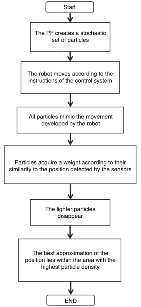
When the programme starts, the robot does not know where it is. However, the actual samples are evenly distributed, and the importance weights are all equal. evenly distributed, and the importance weights are all equal. After a long time, the samples near the current the current position are more likely, and those further away are less likely. The basic algorithm is as follows:
1. Initialise the set of samples. Their locations are evenly distributed and have the same weights.
2. Repeat for each sample until: a) Move the robot a fixed distance and read the sensor. b) For each particle, update the location. c) Assign the importance weights of each particle to the probability of that sensor, and read that new location.
3. Create a collection of samples, by sampling with replacement from the current set of samples, based on their importance weights.
4. Let the group become the current round of samples.

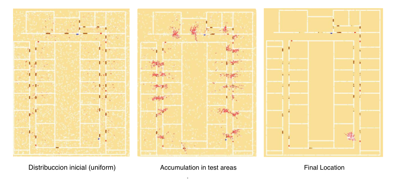
Diagram of the particle filter algorithm

The following figure shows an example of the operation of the particulate filter. At the initial instant the particles are uniformly distributed in the environment. As new observations are obtained, the particles accumulate in probability zones until they converge to the probability zone [5].

Evolution of particles — Probabilistic location model

Videos

Contributors

Contributors: Jose María Cañas, Vladislav Kravchenko
Maintained by David Valladares