Visual Follow Line

Goal

The goal of this exercise is to perform a PID reactive control capable of following the line painted on the racing circuit.

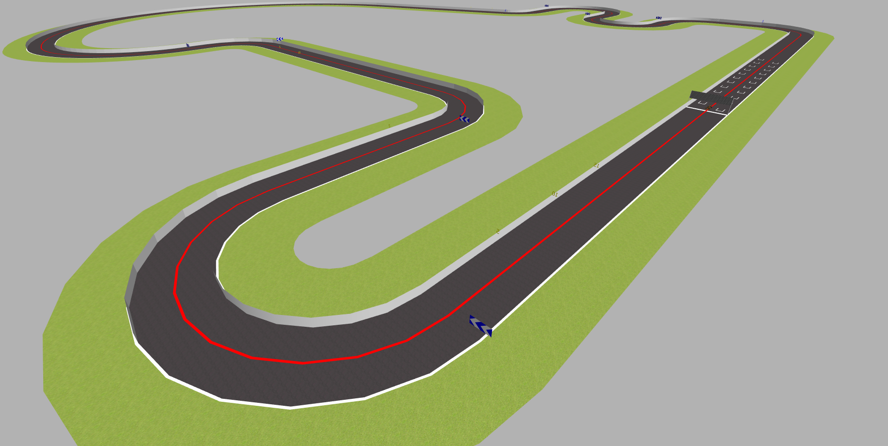
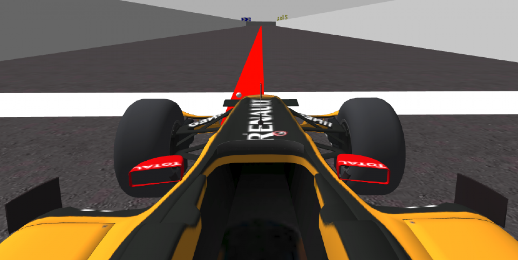
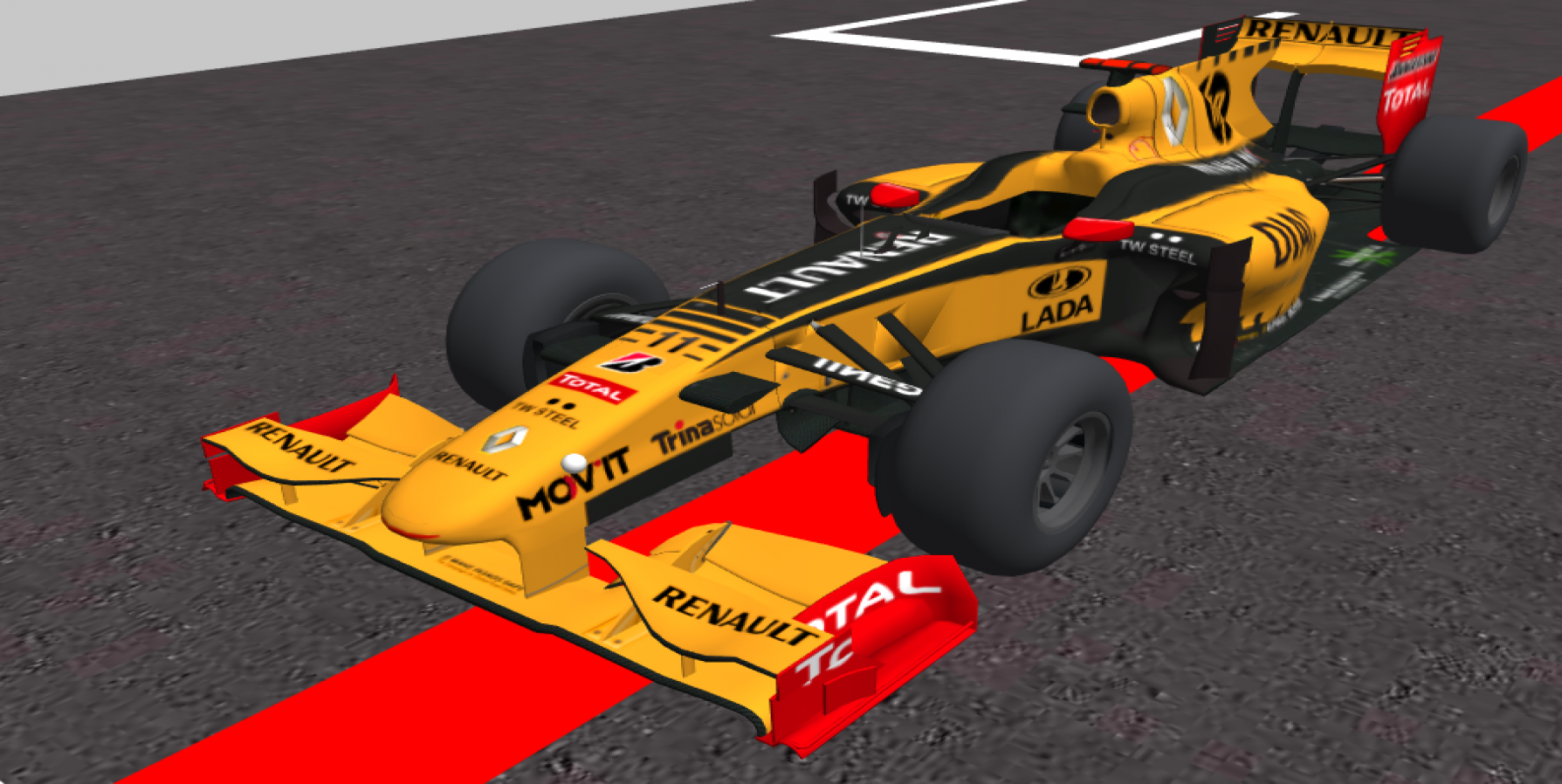
The students will program a Formula1 car in a race circuit to follow the red line in the middle of the road.

Note: If you haven’t, take a look at the user guide to understand how the installation is made, how to launch a RoboticsBackend and how to perform the exercises.

Robot API

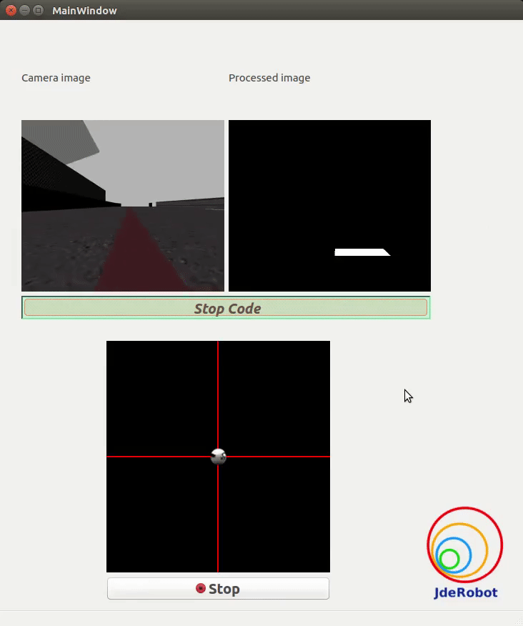
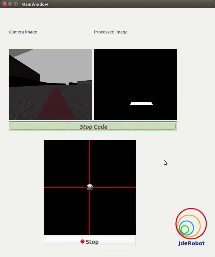
import HAL - to import the HAL(Hardware Abstraction Layer) library class. This class contains the functions that sends and receives information to and from the Hardware(Gazebo).
import GUI - to import the GUI(Graphical User Interface) library class. This class contains the functions used to view the debugging information, like image widgets.
HAL.getImage() - to get the image (BGR8)
HAL.setV(velocity) - to set the linear speed
HAL.setW(velocity) - to set the angular velocity
GUI.showImage(image) - allows you to view a debug image or with relevant information

Theory

PID Control is the main fundamental behind this exercise. To understand PID Control, let us first understand what is Control in general.

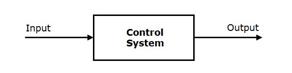
Control System

A system of devices or set of devices, that manages, commands, directs or regulates the behavior of other devices or systems to achieve the desired results. Simply speaking, a system which controls other systems. Control Systems help a robot to execute a set of commands precisely, in the presence of unforeseen errors.

Types of Control System

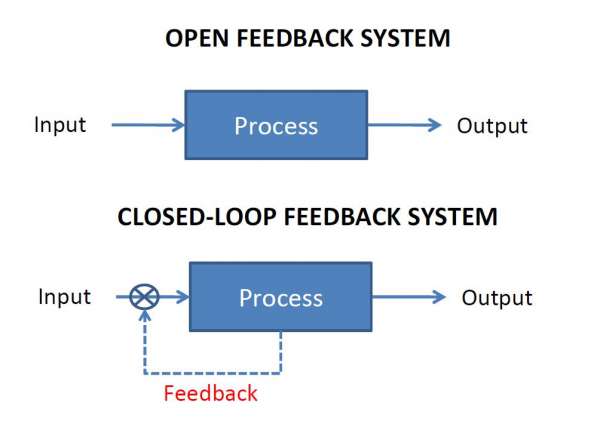
Open Loop Control System

A control system in which the control action is completely independent of the output of the system. A manual control system is on Open Loop System.

Closed Loop Control System

A control system in which the output has an effect on the input quantity in such a manner that the input will adjust itself based on the output generated. An open loop system can be converted to a closed one by providing feedback.

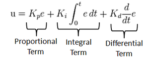
PID Control

A control loop mechanism employing feedback. A PID Controller continuously calculates an error value as the difference between desired output and the current output and applies a correction based on proportional, integral and derivative terms(denoted by P, I, D respectively).

Proportional

Proportional Controller gives an output which is proportional to the current error. The error is multiplied with a proportionality constant to get the output. And hence, is 0 if the error is 0.

Integral

Integral Controller provides a necessary action to eliminate the offset error which is accumulated by the P Controller.It integrates the error over a period of time until the error value reaches to zero.

Derivative

Derivative Controller gives an output depending upon the rate of change or error with respect to time. It gives the kick start for the output thereby increasing system response.

Types of Control Systems — Control Systems and PID

Tuning Methods

In order for the PID equation to work, we need to determine the constants of the equation. There are 3 constants called the gains of the equation. We have 2 main tuning methods for this.

Trial and Error

It is a simple method of PID controller tuning. While system or controller is working, we can tune the controller. In this method, first we have to set Ki and Kd values to zero and increase proportional term (Kp) until system reaches to oscillating behavior. Once it is oscillating, adjust Ki (Integral term) so that oscillations stops and finally adjust D to get fast response.

Zeigler Nichols method

Zeigler-Nichols proposed closed loop methods for tuning the PID controller. Those are continuous cycling method and damped oscillation method. Procedures for both methods are same but oscillation behavior is different. In this, first we have to set the p-controller constant, Kp to a particular value while Ki and Kd values are zero. Proportional gain is increased till system oscillates at constant amplitude.

Real Life Example

Hints

Simple hints provided to help you solve the follow_line exercise.

Detecting the Line to Follow

The first task of the assignment is to detect the line to be followed. This can be achieved easily by filtering the color of the line from the image and applying basic image processing to find the point or line to follow, or in Control terms our Set Point. Refer to these links for more information:

Coding the Controller

The Controller can be designed in various configurations. 3 configurations have been described in detail below:

P Controller The simplest way to do the assignment is using the P Controller. Just find the error which is the difference between our Set Point (The point where our car should be heading) and the Current Output (Where the car is actually heading). Keep adjusting the value of the constant, till we get a value where there occurs no unstable oscillations and no slow response.
PD Controller This is an interesting way to see the effect of Derivative on the Control. For this, we need to calculate the derivative of the output we are receiving. Since, we are dealing with discrete outputs in our case, we simply calculate the difference between our previous error and the present error, then adjust the proportional constant. Adjust this value along with the P gain to get a good result.
PID Controller This is the complete implemented controller. Now, to add the I Controller we need to integrate the output from the point where error was zero, to the present output. While dealing with discrete outputs, we can achieve this using accumulated error. Then, comes the task of adjustment of gain constants till we get our desired result.

Illustrations

examples — Unstable Oscillations (left) - Slow Response (right)

Videos

This solution is an illustration for the Web Templates

Contributors

Contributors: Alberto Martín, Francisco Rivas, Francisco Pérez, Jose María Cañas, Nacho Arranz, Javier Izquierdo.
Maintained by Pankhuri Vanjani and Sakshay Mahna, Javier Izquierdo.