MonteCarlo laser-based robot localization

Goal

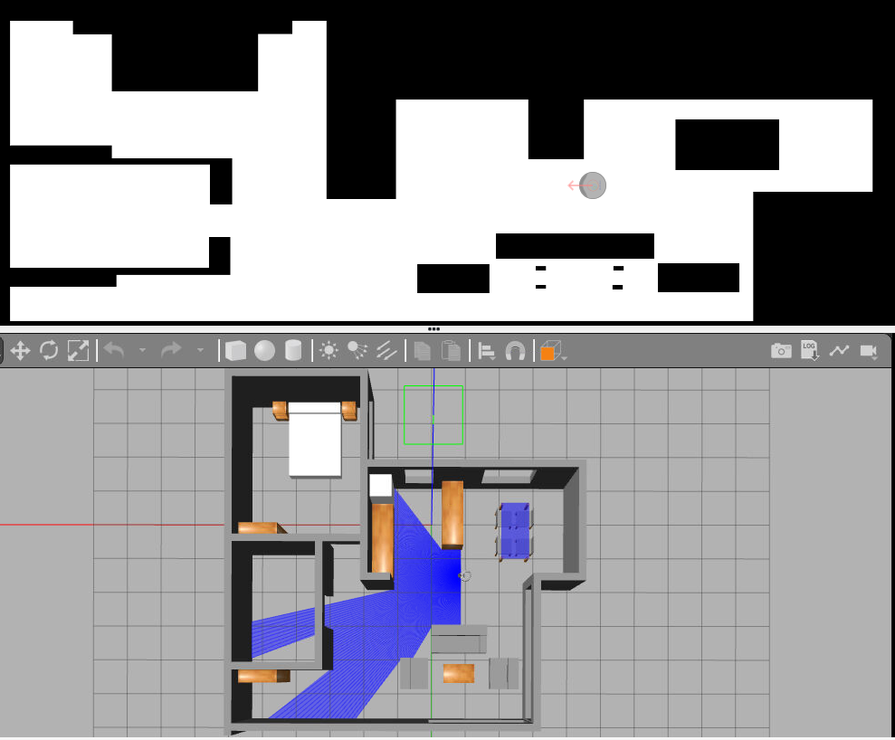
The goal of this exercise is to develop a localization algorithm based on the particle filter using the robot’s laser.

Montecarlo Laser Loc — MonteCarlo Laser Location.

Frequency API

Python

import Frequency - to import the Frequency library class. This class contains the tick function to regulate the execution rate.
Frequency.tick(ideal_rate) - regulates the execution rate to the number of Hz specified. Defaults to 50 Hz.

C++

#include "Frequency.hpp" - to import the Frequency library class. This class contains the tick function to regulate the execution rate.
Frequency freq = Frequency(); - to instanciate the Frequency class.
freq.tick(ideal_rate); - regulates the execution rate to the number of Hz specified. Defaults to 50 Hz.

Robot API

This exercise now supports ROS 2-direct implementation in addition to the original HAL-based approach. Below you’ll find the details for both options.

HAL-based Implementation

Python

import HAL - to import the HAL (Hardware Abstraction Layer) library class. This class contains the functions that receive information from the webcam.
import WebGUI - to import the WebGUI (Web Graphical User Interface) library class. This class contains the functions used to view the debugging information, like image widgets.
HAL.setW() - to set the angular velocity.
HAL.setV() - to set the linear velocity.
HAL.getPose3d().x - to get the X coordinate of the robot.
HAL.getPose3d().y - to get the Y coordinate of the robot.
HAL.getPose3d().yaw - to get the orientation of the robot.
HAL.getOdom().x - to get the approximated X coordinate of the robot (with noise).
HAL.getOdom().y - to get the approximated Y coordinate of the robot (with noise).
HAL.getOdom().yaw - to get the approximated orientation of the robot (with noise).
HAL.getBumperData().state - to establish if the robot has crashed or not. Returns 1 if the robot collides and 0 if it has not crashed.
HAL.getBumperData().bumper - if the robot has crashed, it returns 1 when the crash occurs on center of the robot, 0 when it occurs on its right and 2 if the collision is on its left.
HAL.getLaserData() - to obtain the data of the laser sensor, which consists of 180 pairs of values (0-180º, distance in meters).
WebGUI.showParticles(particles) - shows the particles on the map. Accepts a list of particles as an argument. Each particle must be a list with [position_x, position_y, angle_in_radians, weight]. The values must be in gazebo world coordinate system.
WebGUI.showPosition(x, y, yaw) - shows the estimated user position in the map view in blue. Accepts a list with [position_x, position_y, angle_in_radians]. The values must be in gazebo world coordinate system. The map view will also show the real position of the robot in red, so you can compare how good your algorithm is.
WebGUI.mapToPose(x, y, yaw)- converts a map pixel to gazebo world coordinate system position.
WebGUI.poseToMap(x, y, yaw)- converts a gazebo world coordinate system position to a map pixel.
WebGUI.getMap(url) - Returns a numpy array with the image data in a 3 dimensional array (R, G, B, A). The image is 1012x1012. The instruction to get the map is

array = WebGUI.getMap('/resources/exercises/montecarlo_laser_loc/images/mapgrannyannie.png')

C++

#include "HAL.hpp" - to import the HAL (Hardware Abstraction Layer) library class. This class contains the functions that send and receive information to and from the Hardware (Gazebo).
#include "WebGUI.hpp" - to import the WebGUI (Web Graphical User Interface) library class. This class contains the functions used to view the debugging information, like image widgets.
HAL::set_v(velocity); - sets the linear velocity of the robot. The input is a float. Returns void.
HAL::set_w(velocity); - sets the angular velocity of the robot. The input is a float. Returns void.
HAL::get_pose3d(); - returns the current ground-truth robot pose as a HAL::Pose3d.
HAL::get_pose3d().x; - gets the robot x position in world coordinates (double).
HAL::get_pose3d().y; - gets the robot y position in world coordinates (double).
HAL::get_pose3d().yaw; - gets the robot orientation around the vertical axis in world coordinates (double).
HAL::get_odom(); - returns the noisy odometry pose as a HAL::Pose3d.
HAL::get_odom().x; - gets the noisy odometry x position (double).
HAL::get_odom().y; - gets the noisy odometry y position (double).
HAL::get_odom().yaw; - gets the noisy odometry orientation around the vertical axis (double).
HAL::get_bumper_data(); - returns the bumper sensor data as a HAL::BumperData.
HAL::get_bumper_data().state; - indicates whether the robot has collided (int). A value of 1 means collision and 0 means no collision.
HAL::get_bumper_data().bumper; - indicates which bumper detected the collision (int): 0 for right, 1 for center, and 2 for left.
HAL::get_laser_data(); - returns the laser sensor data as a HAL::LaserData.
HAL::get_laser_data().values; - contains the laser distance readings as a std::vector<float>.
HAL::get_laser_data().minAngle; - minimum laser angle (double).
HAL::get_laser_data().maxAngle; - maximum laser angle (double).
HAL::get_laser_data().minRange; - minimum valid laser range (double).
HAL::get_laser_data().maxRange; - maximum valid laser range (double).
WebGUI::show_position(x, y, angle); - displays the estimated robot position in the WebGUI. The inputs are double values in Gazebo world coordinates. Returns void.
WebGUI::show_particles(particles); - displays the particle set in the WebGUI. The input must be a std::vector<std::vector<double>>, where each particle is represented as [x, y, yaw, weight] in Gazebo world coordinates. Returns void.
WebGUI::pose_to_map(x, y, yaw); - converts a pose from Gazebo world coordinates to map pixel coordinates. The inputs are double values and the function returns a std::vector<double>.
WebGUI::map_to_pose(map_x, map_y, map_yaw); - converts a pose from map pixel coordinates to Gazebo world coordinates. The inputs are double values and the function returns a std::vector<double>.
WebGUI::get_map(url); - returns the map image as a cv::Mat. The input must be a std::string with the map URL.

In order to use the HAL-based controls you must include the following lines:

#include "HAL.hpp"
#include "WebGUI.hpp"
#include "Frequency.hpp"

void exercise() {
    Frequency freq = Frequency();
    // Enter sequential code!

    while (true)
    {
        // Enter iterative code!
        freq.tick();


    }
}

ROS 2-direct Implementation

Use standard ROS 2 topics for direct communication with the simulation.

/cmd_vel - Publish to this topic to set both linear and angular velocities. Message type: geometry_msgs/msg/Twist
/odom - Subscribe to this topic to receive the robot ground-truth odometry. Message type: nav_msgs/msg/Odometry
/odom_noisy - Subscribe to this topic to receive the noisy odometry. Message type: nav_msgs/msg/Odometry
/roombaROS/laser/scan - Subscribe to this topic to receive laser data. Message type: sensor_msgs/msg/LaserScan
/roombaROS/events/right_bumper - Subscribe to this topic to receive right bumper events. Message type depends on the bumper interface used by the exercise.
/roombaROS/events/center_bumper - Subscribe to this topic to receive center bumper events. Message type depends on the bumper interface used by the exercise.
/roombaROS/events/left_bumper - Subscribe to this topic to receive left bumper events. Message type depends on the bumper interface used by the exercise.

For WebGUI debugging:

/webgui/estimated_pose - Publish to this topic to display the estimated robot pose in the WebGUI. Message type: geometry_msgs/msg/PoseStamped
QoS: TRANSIENT_LOCAL, depth 1

/webgui/particles - Publish to this topic to display the particle set in the WebGUI. Message type: geometry_msgs/msg/PoseArray
QoS: TRANSIENT_LOCAL, depth 1

  from geometry_msgs.msg import PoseArray, Pose
  import math

  def publish_particles(self, particles):
      msg = PoseArray()
      msg.header.stamp = self.get_clock().now().to_msg()
      msg.header.frame_id = "map"

      for x, y, yaw in particles:
          pose = Pose()
          pose.position.x = float(x)
          pose.position.y = float(y)

          # Convert yaw → quaternion (2D)
          pose.orientation.z = math.sin(yaw / 2.0)
          pose.orientation.w = math.cos(yaw / 2.0)

          msg.poses.append(pose)

      self.particles_pub.publish(msg)

Python

Note: Ensure this import is included in your script to access the Web GUI functionalities.

import WebGUI - to enable the Web GUI for visualizing camera images.

To have frequency control you need to use standard ROS 2 mechanisms to manage loop timing:

rclpy.spin() - Event-driven execution using callbacks.
rclpy.spin_once() - Single-step processing, often with custom timers.
rclpy.Rate() - Loop-based frequency control.

Note WebGUI already initializes rclpy internally, so this should be taken into account when building a direct ROS 2 solution.

C++

In order to use native ros controls you must include the following lines:

#ifndef USER_NODE
#define USER_NODE

#include "rclcpp/rclcpp.hpp"

class UserNode : public rclcpp::Node {
  // Your class
};

#endif

You must define USER_NODE and a UserNode node class.

To have frequency control you may use a timer and a control function as follows:

  UserNode() : Node("user_node")
  {
    // More subscribers and publishers
    timer_ = create_wall_timer(100ms, std::bind(&UserNode::control_cycle, this));
  };

// More Code

  void control_cycle(){
    // Your function
  };

Types conversion

Laser

import math
import numpy as np

def parse_laser_data(laser_data):
    """ Parses the LaserData object and returns a tuple with two lists:
        1. List of  polar coordinates, with (distance, angle) tuples,
           where the angle is zero at the front of the robot and increases to the left.
        2. List of cartesian (x, y) coordinates, following the ref. system noted below.

        Note: The list of laser values MUST NOT BE EMPTY.
    """
    laser_polar = []  # Laser data in polar coordinates (dist, angle)
    laser_xy = []  # Laser data in cartesian coordinates (x, y)
    for i in range(180):
        # i contains the index of the laser ray, which starts at the robot's right
        # The laser has a resolution of 1 ray / degree
        #
        #                (i=90)
        #                 ^
        #                 |x
        #             y   |
        # (i=180)    <----R      (i=0)

        # Extract the distance at index i
        dist = laser_data.values[i]
        # The final angle is centered (zeroed) at the front of the robot.
        angle = math.radians(i - 90)
        laser_polar += [(dist, angle)]
        # Compute x, y coordinates from distance and angle
        x = dist * math.cos(angle)
        y = dist * math.sin(angle)
        laser_xy += [(x, y)]
    return laser_polar, laser_xy

# Usage
laser_data = HAL.getLaserData()
if len(laser_data.values) > 0:
    laser_polar, laser_xy = parse_laser_data(laser_data)

Theory

Probabilistic localisation seeks to estimate the position of the robot and the model of the surrounding environment:

A. Probabilistic motion model. Due to various sources of noise (bumps, friction, imperfections of the robot, etc.) it is very difficult to predict the movement of the robot accurately. Therefore, it would be more convenient to describe this movement by means of a probability function, which will move with the robot’s movements [1].
B. Probabilistic model of sensory observation. It is related to the sensor measurements at each instant of time. This model is built by taking observations at known positions in the environment and calculating the probability that the robot is in each of these positions [2].
C. Probability fusion. This consists of accumulating the information obtained at each time instant, something that can be done using Bayes’ theorem. This fusion achieves that in each observation some modes of the probability function go up and others go down, so that as the number of iterations advances, the probability will be concentrated in only one of the modes, which will indicate the position of the robot [3].

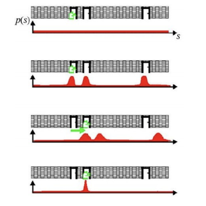
The following figure shows an example of probabilistic localisation. In the first phase, the robot does not know its initial state, the initial probability distribution is uniform. In the second phase, the robot is looking at a door, the sensory observation model determines that there are three zones or modes with equal probability of being the zone where the robot is. In the third phase, the robot is moving forward so the probabilistic motion model is applied, the probability distribution should move the same distance that the robot has moved, but as estimating the motion is difficult, what is done is to smooth it. In the last phase, the robot detects another door and this observation is merged with the accumulated information. This causes the probability to concentrate on a single possible area where it can be found, and thus ends the global localisation process.

Monte Carlo

Monte Carlo localisation is based on a collection of particles or samples. Particle filters allow the localisation problem to be solved by representing the a posteriori probability function, which estimates the most likely positions of the robot. The a posteriori probability distribution is sampled, in a way where each sample is called a particle [4].
Each particle represents a state (position) at time t and has an associated weight. At each movement of the robot, they perform a correction and decrease the accumulated error. After a number of iterations, the particles are grouped in the zones with the highest probability, until they converge to a single zone, which corresponds to the robot’s position.
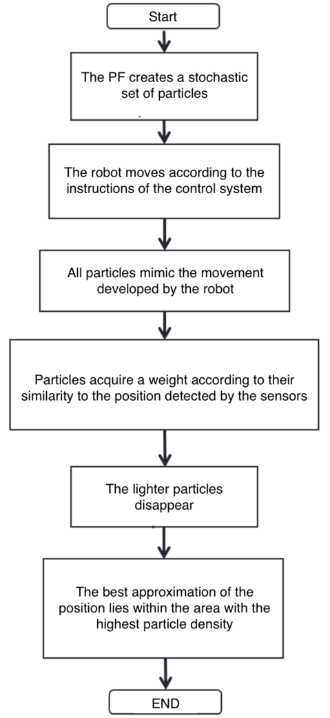
When the program starts, the robot does not know where it is. However, the actual samples are evenly distributed and the importance weights are all equal. After a long time, the samples near the current position have a higher probability, and those further away have a lower probability. The basic algorithm is as follows:
1. Initialise the set of samples. Their locations are evenly distributed and have the same weights.
2. Repeat for each sample until: a) Move the robot a fixed distance and read the sensor. b) For each particle, update the location. c) Assign the importance weights of each particle to the probability of that sensor, and read that new location.
3. Create a collection of samples, by sampling with replacements from the current set of samples, based on their importance weights.
4. Let the group become the current round of samples.

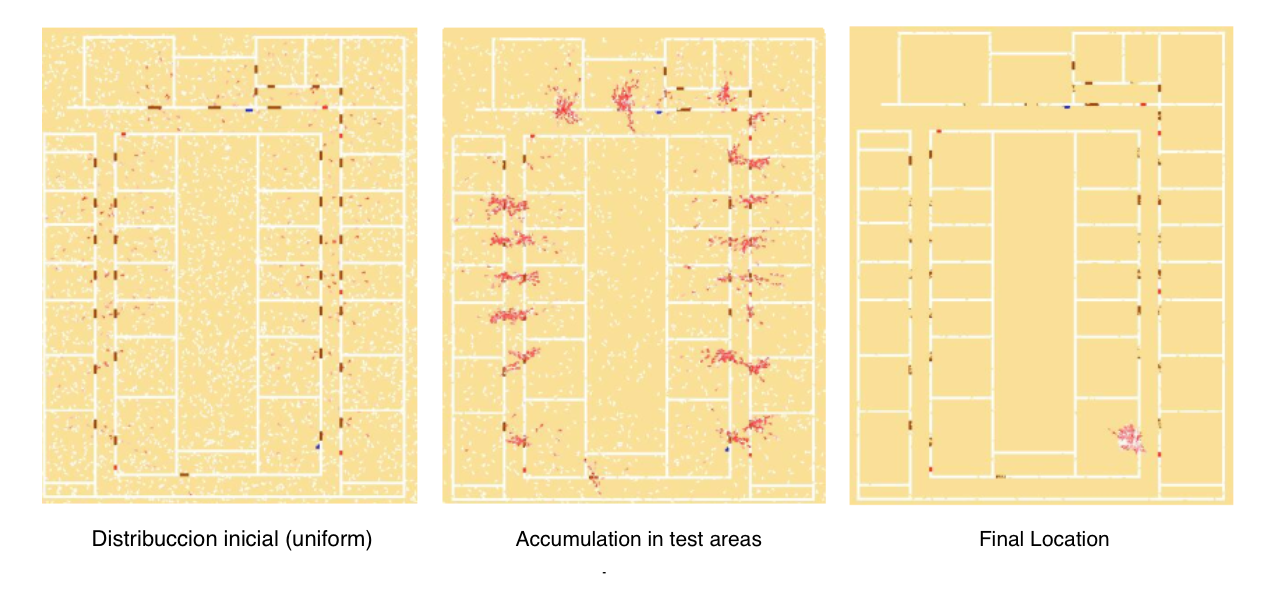
Diagram of the particle filter algorithm

The following figure shows an example of the operation of the particle filter. At the initial instant the particles are uniformly distributed in the environment. As new observations are obtained, the particles accumulate in probability zones until they converge to the probability zone [5].

Evolution of particles — Probabilistic location model

Demonstrative video of the solution

Contributors

Contributors: Jose María Cañas, Vladislav Kravchenko
Maintained by David Valladares

Goal

Frequency API

Python

C++

Robot API

HAL-based Implementation

Python

C++

ROS 2-direct Implementation

Python

C++

Types conversion

Laser

Theory

Monte Carlo

Demonstrative video of the solution

Contributors

References