Laser Line Mapping
Goal
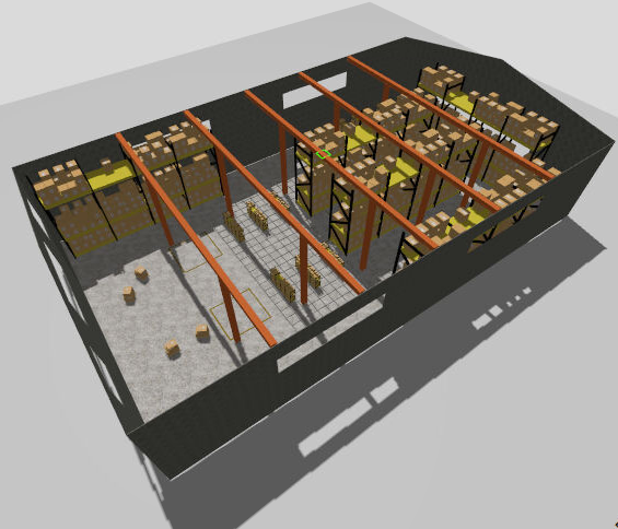
The goal of this exercise is to implement a laser-based line segment mapping algorithm that builds a geometric map of a warehouse environment using a mobile robot equipped with a 2D laser scanner.
The robot must be able to:
- Process raw laser scan data and project it into world coordinates
- Extract line segments from the laser point cloud
- Maintain a consistent global map by merging new detections with existing segments
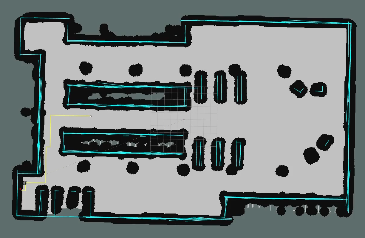
- Visualize the resulting segment map in real time on the WebGUI
Frequency API
Python
import Frequency- to import the Frequency library class. This class contains the tick function to regulate the execution rate.Frequency.tick(ideal_rate)- regulates the execution rate to the number of Hz specified. Defaults to 50 Hz.
C++
#include "Frequency.hpp"- to import the Frequency library class. This class contains the tick function to regulate the execution rate.Frequency freq = Frequency();- to instanciate the Frequency class.freq.tick(ideal_rate);- regulates the execution rate to the number of Hz specified. Defaults to 50 Hz.
Robot API
This exercise now supports ROS 2-direct implementation in addition to the original HAL-based approach. Below you’ll find the details for both options.
HAL-based Implementation
Python
import HAL- to import the HAL library class. This class contains the functions that receive information from the sensors or work with the actuators.import WebGUI as GUI- to import the WebGUI (Web Graphical User Interface) library class. This class contains the functions used to visualize the segment map.HAL.getPose3d().x- to get the X position of the robot in world coordinates (meters).HAL.getPose3d().y- to get the Y position of the robot in world coordinates (meters).HAL.getPose3d().yaw- to get the orientation of the robot in radians.HAL.setV(v)- to set the linear velocity of the robot (m/s).HAL.setW(w)- to set the angular velocity of the robot (rad/s).HAL.getLaserData()- returns the laser scan data object with the following fields:.values- list of range measurements (meters).minAngle- minimum scan angle (radians).maxAngle- maximum scan angle (radians).minRange- minimum valid range (meters).maxRange- maximum valid range (meters)
GUI.addLine(color, p1, p2)- draws a line segment on the map canvas between two world-coordinate points.coloris an RGB tuple e.g.(0, 200, 255).p1andp2are world-coordinate tuples(x, y)in meters. Segments accumulate and persist on screen untilclearSegments()is called.GUI.clearSegments()- clears all segments previously drawn on the map canvas.GUI.getMap()- returns the warehouse map as a NumPy array (RGB).HAL.worldToMap(x, y)/GUI.worldToMap(x, y)- converts world coordinates (meters) to map pixel coordinates(col, row). Available on bothHALandGUI.HAL.mapToWorld(col, row)/GUI.mapToWorld(col, row)- converts map pixel coordinates(col, row)to world coordinates(x, y)in meters. Available on bothHALandGUI.
C++
#include "HAL.hpp"- to import the HAL (Hardware Abstraction Layer) library class. This class contains the functions that send and receive information to and from the Hardware (Gazebo).#include "WebGUI.hpp"- to import the WebGUI (Web Graphical User Interface) library class. This class contains the functions used to visualize the segment map.HAL::set_v(velocity);- sets the linear velocity of the robot. The input is afloat. Returnsvoid.HAL::set_w(velocity);- sets the angular velocity of the robot. The input is afloat. Returnsvoid.HAL::get_pose3d();- returns the ground-truth robot pose as aHAL::Pose3d.HAL::get_pose3d().x;- gets the robot x position in world coordinates (double).HAL::get_pose3d().y;- gets the robot y position in world coordinates (double).HAL::get_pose3d().yaw;- gets the robot orientation around the vertical axis in world coordinates (double).HAL::get_laser_data();- returns the laser sensor data as aHAL::LaserData.HAL::get_laser_data().values;- contains the laser distance readings as astd::vector<float>.HAL::get_laser_data().minAngle;- minimum laser angle (double).HAL::get_laser_data().maxAngle;- maximum laser angle (double).HAL::get_laser_data().minRange;- minimum valid laser range (double).HAL::get_laser_data().maxRange;- maximum valid laser range (double).WebGUI::get_map(url);- loads the warehouse map from disk and returns it as a colourcv::Mat.urlis the map path,/resources/exercises/line_mapper/images/warehouse.png.WebGUI::add_line(color, p1, p2);- draws a line segment on the map canvas between two world-coordinate points.coloris astd::vector<int>{r, g, b},p1andp2arestd::vector<double>{x, y}. Segments accumulate and persist untilclear_segments()is called.WebGUI::clear_segments();- clears all segments previously drawn on the map canvas.WebGUI::world_to_map(x, y);- converts world coordinates (metres) to map pixel coordinates. Returns astd::vector<int>{col, row}.WebGUI::map_to_world(col, row);- converts map pixel coordinates to world coordinates (metres). Returns astd::vector<double>{x, y}.
In order to use the HAL-based controls you must include the following lines:
#include "HAL.hpp"
#include "WebGUI.hpp"
#include "Frequency.hpp"

void exercise() {
    Frequency freq = Frequency();
    // Enter sequential code!

    while (true)
    {
        // Enter iterative code!
        freq.tick();


    }
}
ROS 2-direct Implementation
Use standard ROS 2 topics for direct communication with the simulation.
-
/cmd_vel- Publish to this topic to set both linear and angular velocities. Message type:geometry_msgs/msg/Twist -
/odom- Subscribe to this topic to receive the robot odometry, from which the pose (x,y,yaw) can be extracted. Message type:nav_msgs/msg/Odometry -
/scan- Subscribe to this topic to receive the laser scan. Message type:sensor_msgs/msg/LaserScan
For map debugging, the /webgui/* topics mirror the WebGUI drawing methods:
-
/webgui/lines- Publish to this topic to draw the segment map, equivalent toaddLine. Message type:std_msgs/msg/String, containing a JSON array of entries{"color": [r, g, b], "p1": [x, y], "p2": [x, y]}in world coordinates. Each published message replaces the full segment set shown in the GUI, so a solution should publish the complete list of current segments on every update rather than appending one segment at a time. -
/webgui/clear_segments- Publish to this topic to clear all segments previously drawn on the map canvas, equivalent toclearSegments. Message type:std_msgs/msg/Empty.
All /webgui/* topics use the default QoS profile with a history depth of 10.
Loading the map image itself is not exposed as a topic, so a ROS 2-direct solution should read /resources/exercises/line_mapper/images/warehouse.png directly from disk and apply the same world-to-map transform used by HAL and WebGUI, resolution 0.05 m/px, origin (-15.0, -25.0), size 1002x603 px.
Python
Note: Ensure this import is included in your script to access the Web GUI functionalities.
import WebGUI - to enable the Web GUI for visualizing the segment map.
To have frequency control you need to use standard ROS 2 mechanisms to manage loop timing:
rclpy.spin()- Event-driven execution using callbacks.rclpy.spin_once()- Single-step processing, often with custom timers.rclpy.Rate()- Loop-based frequency control.
Note
WebGUI already initializes rclpy internally, so this should be taken into account when building a direct ROS 2 solution.
C++
In order to use direct ros controls you must include the following lines:
#ifndef USER_NODE
#define USER_NODE

#include "rclcpp/rclcpp.hpp"

class UserNode : public rclcpp::Node {
  // Your class
};

#endif
You must define USER_NODE and a UserNode node class.
To have frequency control you may use a timer and a control function as follows:
  UserNode() : Node("user_node")
  {
    // More subscribers and publishers
    timer_ = create_wall_timer(100ms, std::bind(&UserNode::control_cycle, this));
  };

// More Code

  void control_cycle(){
    // Your function
  };
Odometry Noise Variants
This exercise provides three universe variants to test the robustness of the mapping algorithm under different odometry noise conditions:
- Rover 4wd Warehouse — no odometry noise. The robot pose is perfectly accurate. The resulting segment map should closely match the real geometry of the warehouse.
- Rover 4wd Warehouse Low Noise — low odometry noise. Small drift accumulates over time. The segment map will show minor misalignments between segments observed from different robot positions.
- Rover 4wd Warehouse High Noise — high odometry noise. Significant drift accumulates. The segment map will show visible inconsistencies as the robot moves further from its starting position.
Comparing the maps produced across the three variants illustrates the impact of odometry error on geometric mapping and motivates the use of localization or loop closure techniques in real systems.
Theory
Laser Scan Projection
The raw laser data consists of range measurements at known angles relative to the robot’s laser frame. To build a world-frame map, each range measurement must be transformed into world coordinates using the robot’s current pose.
Each laser beam is described by a distance and an angle relative to the robot. The angle of each beam is computed from the scan parameters:
angle_increment = (maxAngle - minAngle) / num_beams
angle_i = minAngle + i * angle_increment
The Cartesian coordinates of the beam endpoint in the laser frame are:
lx = dist * cos(angle_i)
ly = dist * sin(angle_i)
These local coordinates are then rotated into the robot body frame and projected into world coordinates using the robot pose (x, y, yaw).
The laser sensor is typically mounted at an offset from the robot’s geometric center. This offset must be added to the robot position before projecting the scan points into the world frame.
Line Extraction from Point Clouds
Once the laser scan is projected into world coordinates, the resulting point cloud can be processed to extract line segments that represent the flat surfaces and walls in the environment.
A typical pipeline consists of three stages:
1. Line fitting
A line model is fitted to a subset of points. The goal is to find the line that best explains the maximum number of nearby points. RANSAC (Random Sample Consensus) is a classical approach: it randomly samples pairs of points, fits a line through them, and counts how many other points lie within a distance threshold. The iteration with the most inliers is kept.
2. Segment extraction
The inlier points are projected onto the fitted line direction and sorted. Gaps larger than a threshold break the sorted sequence into individual segments. Segments that are too short or too long are discarded.
3. Map update (merge or add)
Each extracted segment is compared against the existing global map. If a compatible segment already exists — similar orientation, close distance, overlapping position — the two are merged into an extended segment. Otherwise the new segment is added to the map.
Segment Compatibility
Two segments are considered compatible if they satisfy a set of geometric criteria simultaneously:
- Their orientations differ by less than an angular threshold.
- The midpoint of the new segment lies close to the infinite line supporting the existing segment.
- The endpoints of both segments are spatially close enough to suggest they describe the same physical surface.
Segment Lifetime
In a noisy environment, false detections will appear and disappear. A robust mapper should filter them out. Two common strategies are:
-
Hit counting: each segment accumulates a counter each time a compatible observation confirms it. Only segments with enough confirmations are rendered in the GUI. Segments that stop receiving confirmations are eventually removed.
-
Negative evidence: if the laser beam passes through the location of a segment without detecting an obstacle, this counts as evidence against it. Segments that accumulate enough such misses are deleted.
Effect of Odometry Noise
All coordinate transformations in this exercise rely on the robot’s pose estimate provided by HAL.getPose3d(). Any error in this estimate directly degrades the quality of the map. As the robot moves further from its starting position, small errors in each pose estimate accumulate, causing segments observed from different locations to appear misaligned.
The three universe variants (no noise, low noise, high noise) allow the user to observe this degradation experimentally and understand the fundamental relationship between localization accuracy and map quality.
Videos
Contributors
- Contributors: Carlos Iglesias
- Maintained by Carlos Iglesias