Optical Flow Teleop

Goal

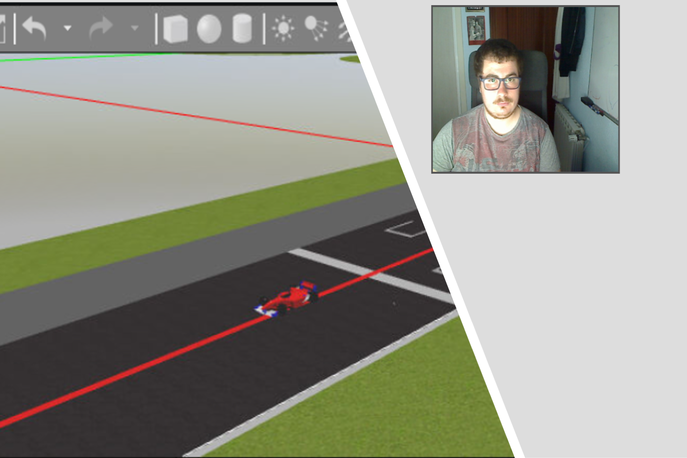
In this practice the intention is to develop an optical flow algorithm to teleoperate the robot using the images obtained from a webcam.

Instructions

This is the preferred way for running the exercise.

Installation

Clone the Robotics Academy repository on your local machine

git clone https://github.com/JdeRobot/RoboticsAcademy

Download Docker. Windows users should choose WSL 2 backend Docker installation if possible, as it has better performance than Hyper-V.
Pull the current distribution of Robotics Academy Docker Image

docker pull jderobot/robotics-academy:latest

How to perform the exercise?

Start a new docker container of the image and keep it running in the background. It is necessary to map the port where the camera is located to the docker container.
For ubuntu: The port to map will be in /dev/videoX , you should check the number where your camera is connected. For exaple /dev/video0

docker run --rm -it -p 7164:7164 -p 2303:2303 -p 1905:1905 -p 8765:8765 -p 6080:6080 -p 1108:1108 --device /dev/video0:/dev/video0 jderobot/robotics-academy:latest

For MacOs and Windows: A number of configurations must be made in order to map the ports. You can visit this documentation for it.
On the local machine navigate to 127.0.0.1:7164/ in the browser and choose the desired exercise.
Wait for the Connect button to turn green and display “Connected”. Click on the “Launch” button and wait for some time until an alert appears with the message Connection Established and button displays “Ready”.
The exercise can be used after the alert.

Where to insert the code?

In the launched webpage, type your code in the text editor,

from GUI import GUI
from HAL import HAL
# Enter sequential code!


while True:
    # Enter iterative code!

Using the Interface

Control Buttons: The control buttons enable the control of the interface. Play button sends the code written by User to the Image. Stop button stops the code that is currently running on the Image. Save button saves the code on the local machine. Load button loads the code from the local machine. Reset button resets the simulation (primarily, the image of the camera).
Brain and GUI Frequency: This input shows the running frequency of the iterative part of the code (under the while True:). A smaller value implies the code runs less number of times. A higher value implies the code runs a large number of times. The numerator is the one set as the Measured Frequency who is the one measured by the computer (a frequency of execution the computer is able to maintain despite the commanded one) and the input (denominator) is the Target Frequency which is the desired frequency by the student. The student should adjust the Target Frequency according to the Measured Frequency.
RTF (Real Time Factor): The RTF defines how much real time passes with each step of simulation time. A RTF of 1 implies that simulation time is passing at the same speed as real time. The lower the value the slower the simulation will run, which will vary depending on the computer.
Pseudo Console: This shows the error messages related to the student’s code that is sent. In order to print certain debugging information on this console. The student is provided with console.print() similar to print() command in the Python Interpreter.

Robot API

from HAL import HAL - to import the HAL library class. This class contains the functions that receives information from the webcam.
from GUI import GUI - to import the GUI (Graphical User Interface) library class. This class contains the functions used to view the debugging information, like image widgets.
HAL.getImage() - to get the image
GUI.showImage() - allows you to view a debug image or with relevant information
HAL.motors.sendV() - to set the linear speed
HAL.motors.sendW() - to set the angular velocity

##Videos

Theory

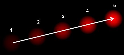
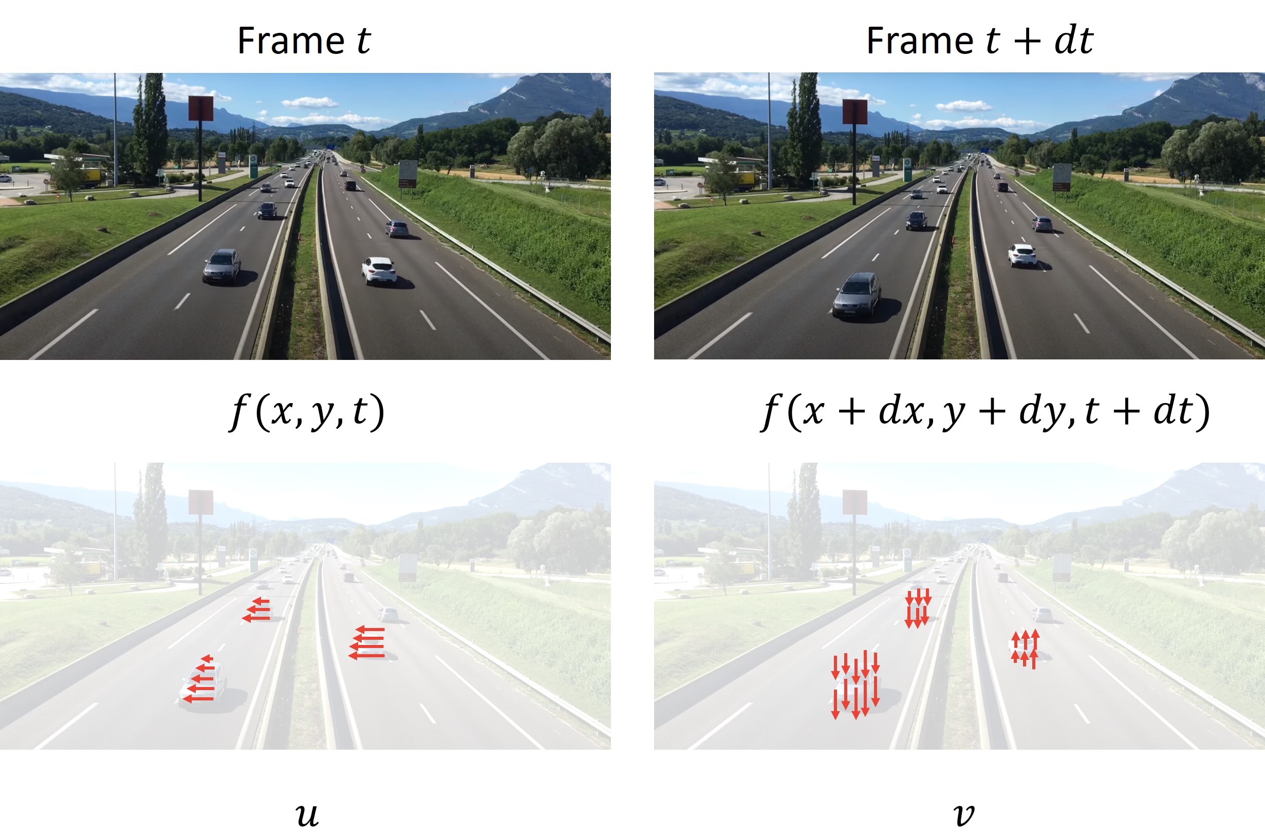
Optical flow is the pattern of apparent motion of image objects between two consecutive frames caused by the movement of object or camera. It is 2D vector field where each vector is a displacement vector showing the movement of points from first frame to second. Consider the image below:

Optical flow works on several assumptions:
1. The pixel intensities of an object do not change between consecutive frames.
2. Neighbouring pixels have similar motion.

Optical Flow Example — Example of optical flow motion estimation

Optical flow has many applications in areas like:
- Structure from Motion
- Video Compression
- Video Stabilization

Contributors

Contributors: Jose María Cañas, David Valladares
Maintained by David Valladares