3D Reconstruction

Goal

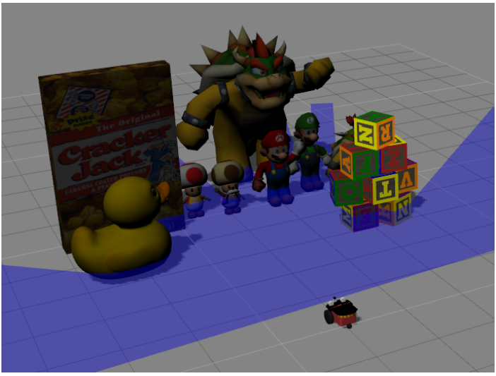
In this practice, the intention is to program the necessary logic to allow kobuki robot to generate a 3D reconstruction of the scene that it is receiving throughout its left and right cameras.

Note: If you haven’t, take a look at the user guide to understand how the installation is made, how to launch a RoboticsBackend and how to perform the exercises.

Robot API

from HAL import HAL - to import the HAL(Hardware Abstraction Layer) library class. This class contains the functions that sends and receives information to and from the Hardware(Gazebo).
from GUI import GUI - to import the GUI(Graphical User Interface) library class. This class contains the functions used to view the debugging information, like image widgets.
HAL.getImage('left') - to get the left image
HAL.getImage('right') - to get the right image
HAL.getCameraPosition('left') - to get the left camera position from ROS Driver Camera
HAL.getCameraPosition('right') - to get the right camera position from ROS Driver Camera
HAL.graficToOptical('left', point2d) - to transform the Image Coordinate System to the Camera System
HAL.backproject('left', point2d) - to backprojects the 2D Image Point into 3D Point Space
HAL.project('left', point3d) - to backprojects a 3D Point Space into the 2D Image Point
HAL.opticalToGrafic('left', point2d) - to transform the Camera System to the Image Coordinate System
HAL.project3DScene(point3d) - to transform 3D Point Space after triangulation to the 3D Point Viewer
GUI.ShowNewPoints(points) - to plot a array of plots in the 3D visor
GUI.ShowAllPoints(points) - to clear the 3D visor and plot new array of plots
GUI.ClearAllPoints() - to clear the 3D visor
GUI.showImageMatching(x1, y1, x2, y2) - to plot the matching between two images
GUI.showImages(imageLeft,imageRight,True) - allows you to view a debug images or with relevant information

def algorithm(self):
	#GETTING THE IMAGES
	# imageR = self.getImage('right')
	# imageL = self.getImage('left')

	#EXAMPLE OF HOW TO PLOT A RED COLORED POINT
	# position = [1.0, 0.0, 0.0]	X, Y, Z
	# color = [1.0, 0.0, 0.0]	R, G, B
	# self.point.plotPoint(position, color) 

3D Viewer

Mouse

Mouse wheel: if it is rotated forward, the zoom will increase. If it is rotated backwards, it will zoom out.
Right mouse button: if it is held down and the mouse is dragged, the content of the window will move in the same direction.
Left mouse button: if it is held down and the mouse is dragged, the content of the window will rotate in the same direction.

Keyboard

Direction keys and Numerical keypad: the content of the window will move in the same direction of the key.
Minus keys: if it is held down, it will zoom out.
Plus keys: if it is held down, the zoom will increase.

Videos

Application Programming Interface

self.getImage('left') - to get the left image
self.getImage('right') - to get the right image
self.point.PlotPoint(position, color) - to plot the point in the 3d tool

Navigating the GUI Interface

Mouse based: Hold and drag to move around the environment. Scroll to zoom in or out

Keyboard based: Arrow keys to move around the environment. W and S keys to zoom in or out

Theory

In computer vision and computer graphics, 3D reconstruction is the process of determining an object’s 3D profile, as well as knowing the 3D coordinate of any point on the profile. Reconstruction can be achieved as follows:

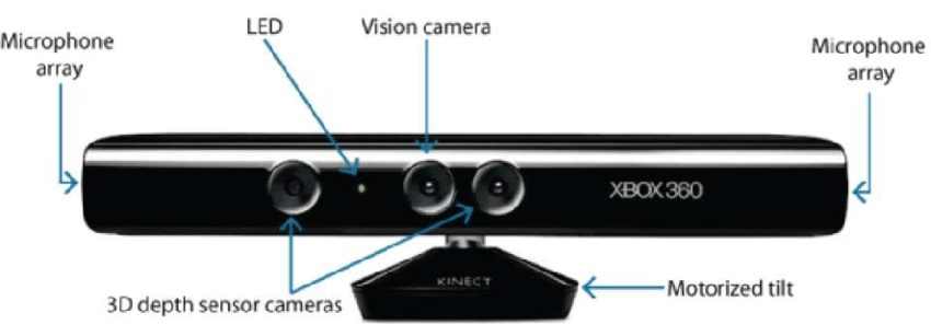
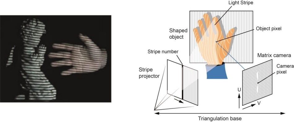
Hardware Based: Hardware based approach requires us to utilize the hardware specific to the reconstruction task. Use of structured light, laser range finder, depth gauge and radiometric methods are some examples.

Microsoft Kinect — Hardware based 3D Reconstruction

3D Imaging — Hardware based 3D Reconstruction

Software Based: Software based approach relies on the computation abilities of the computer to determine the 3D properties of the object. Shape from shading, texture, stereo vision and homography are some good methods.

In this exercise our main aim is to carry out 3d reconstruction using Software based approach, particularly stereo vision 3d reconstruction.

Epipolar Geometry

When two cameras view a 3D scene from two different positions, there are a number of geometric relations between the 3D points and their projections onto the 2D images that lead to constraints between the image points. The study of these properties and constraints is called Epipolar Geometries. The image and explanation below may generalize the idea:

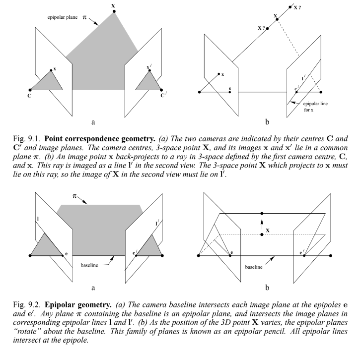
Suppose a point X in 3d space is imaged in two views, at x in the first and x' in the second. Backprojecting the rays to their camera centers through the image planes, we obtain a plane surface, denoted by π.

Supposing now that we know only x, we may ask how the corresponding point x' is constrained. The plane π is determined by the baseline(line connecting the camera centers) and the ray defined by x. From above, we know that the ray corresponding to the unknown point x' lies in π, hence the point x' lies on the line of intersection l' of π with second image plane. This line is called the epipolar line corresponding to x. This relation helps us to reduce the search space of the point in right image, from a plane to a line. Some important definitions to note are:

The epipole is the point of intersection of the line joining the camera centers (the baseline) with the image plane.
An epipolar plane is a plane containing the baseline.
An epipolar line is the intersection of the epipolar plane with the image plane.

Stereo Reconstruction

Stereo reconstruction is a special case of the above 3d reconstruction where the two image planes are parallel to each other and equally distant from the 3d point we want to plot.

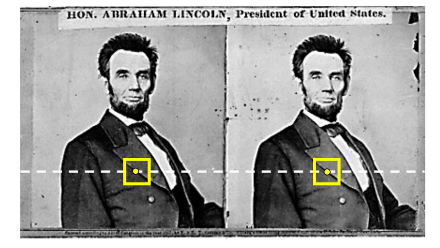
In this case the epipolar line for both the image planes are same, and are parallel to the width of the planes, simplifying our constraint better.

3D Reconstruction Algorithm

The reconstruction algorithm consists of 3 steps:

Detect the feature points in one image plane
Detect the feature point corresponding the one found above
Triangulate the point in 3d space

Let’s look at them one by one

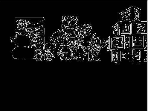
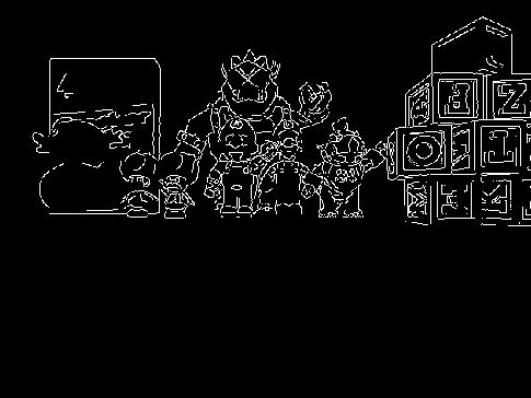
Feature Point Detection

Feature Point Detection is a vast area of study where several algorithms are already studied. Harris Corner Detection and Shi-Tomasi algorithms use eigen values to get a good feature point. But, the problem is we need a lot of points for 3D Reconstruction, and these algorithms won’t be able to provide us with such a large number of feature points.

Therefore, we use edge points as our feature points. There may be ambiguity in their detection in the next stage of the algorithm. But, our problem is solved by taking edges as the feature points. One really cool edge detector is Canny Edge Detection Algorithm. The algorithm is quite simple and reliable in terms of generating the edges.

Feature Point Extraction

The use of the epipolar constraint really simplifies the time complexity of our algorithm. For general 3d reconstruction problems, we have to generate an epipolar line for every point in one image frame, and then search in that sample space the corresponding point in the other image frame. The generation of epipolar line is also very easy in our case, it is just the parallel line iterpolation from left image to right image plane.

Checking the correspondence between images involves many algorithms, like Sum of Squared Differences or Energy Minimization. Without going much deep, using a simple Correlation filter also suffices our use case.

Triangulation

Triangulation in simple terms is just calculating where the 3d point is going to lie using the two determined points in the image planes.

In reality, the position of the image points cannot be measured exactly. For general cameras, there may be geometric or physical distortions. Therefore, a lot of mathematics goes behind minimizing that error and calculating the most accurate 3d point projection. Refer to this link for a simple model.

Hints

Simple hints provided to help you solve the 3d_reconstruction exercise. The OpenCV library is used extensively for this exercise.

Setup

Using the exercise API, we can easily retrieve the images. Also, after getting the images, it is a good idea to perform bilateral filtering on the images, because there are some extra details that need not be included during the 3d reconstruction. Check out the illustrations for the effects of performing the bilateral filtering.

Calculating Correspondences

OpenCV already has built-in correlation filters which can be called through matchTemplate(). Take care of extreme cases like edges and corners.

One good observation is that the points on left will have correspondence in the left part and the points on right will have correspondence in the right part. Using this observation, we can easily speed up the calculation of correspondence.

Plotting the Points

Either manual or OpenCV based function triangulatePoints works good for triangulation. Just take care of all the matrix shapes and sizes while carrying out the algebraic implementations.

Keep in mind the difference between simple 3D coordinates and homogenous 4D coordinates. Check out this video for details. Simply dividing the complete 4d vector by its 4th coordinate gives us the 3d coordinates.

Due to varied implementations of users, the user may have to adjust the scale and offset of the triangulated points in order to make them visible and representable in the GUI interface. Downscaling the 3D coordinate vector by a value between 500 to 1000 works well. Also an offset of 0 to 8 works good.

Illustrations

Without Bilateral Filtering — Illustrations

With Bilateral Filtering — Illustrations

Contributors

Contributors: Alberto Martín, Francisco Rivas, Francisco Pérez, Jose María Cañas, Nacho Arranz.
Maintained by Jessica Fernández, Vanessa Fernández and David Valladares.