Local navigation with VFF

Goal

The objective of this exercise is to implement the logic of the VFF navigation algorithm.

In navigation using a VFF (Virtual Force Field):

Each object in the environment generates a repulsion force against the robot.
The destination generates a force of attraction which pulls the robot.

This makes it possible for the robot to go towards the target, distancing itself from the obstacles, so that its direction is the vector sum of all forces.

The solution can integrate one or more of the following difficulty increasing goals, as well as any other one that occurs to you:

Go as quickly as possible.
Choose the safest route.
Obstacles in movement.
Robustness in situations of indecision (zero vector sum).

Frequency API

Python

import Frequency - to import the Frequency library class. This class contains the tick function to regulate the execution rate.
Frequency.tick(ideal_rate) - regulates the execution rate to the number of Hz specified. Defaults to 50 Hz.

C++

#include "Frequency.hpp" - to import the Frequency library class. This class contains the tick function to regulate the execution rate.
Frequency freq = Frequency(); - to instanciate the Frequency class.
freq.tick(ideal_rate); - regulates the execution rate to the number of Hz specified. Defaults to 50 Hz.

Robot API

This exercise now supports ROS 2-direct implementation in addition to the original HAL-based approach. Below you’ll find the details for both options.

HAL-based Implementation

Python

import HAL - to import the HAL (Hardware Abstraction Layer) library class. This class contains the functions that send and receive information to and from the Hardware (Gazebo).
import WebGUI - to import the WebGUI (Web Graphical User Interface) library class. This class contains the functions used to view the debugging information, like image widgets.
HAL.getPose3d().x - to get the position of the robot (x coordinate)
HAL.getPose3d().y - to obtain the position of the robot (y coordinate)
HAL.getPose3d().yaw - to get the orientation of the robot with regarding the map
HAL.getLaserData() - to obtain laser sensor data It is composed of 180 pairs of values: (0-180º distance in meters)
HAL.setV() - to set the linear speed
HAL.setW() - to set the angular velocity
WebGUI.getNextTarget() - to obtain the next target object on the scenario.
WebGUI.setTargetx - sets the x coordinate of the target on the WebGUI.
WebGUI.setTargety - sets the y coordinate of the target on the WebGUI.
WebGUI.showForces - shows the forces being appliend on the car in real time.

To access the target ‘x’ and ‘y’ coordinates use (target is the object obtained from WebGUI.getNextTarget):

target.getPose().x - to obtain the x position of the target
target.getPose().y - to obtain the y position of the target

Own API

To simplify the exercise, the implementation of control points is offered. To use it, only two actions must be carried out:

Obtain the following point:

currentTarget = WebGUI.getNextTarget()
Mark it as visited when necessary:

currentTarget.setReached(True)

Debugging

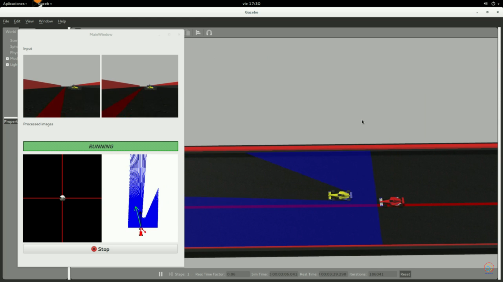
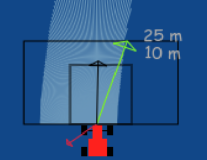
The graphical interface (WebGUI) allows the visualization of each of the vectors of calculated forces. There is a function for this purpose:

# Car direction  (green line in the image below)
carForce = [2.0, 0.0]
# Obstacles direction (red line in the image below)
obsForce = [0.0, 2.0]
# Average direction (black line in the image below)
avgForce = [-2.0, 0.0]

WebGUI.showForces(carForce, obsForce, avgForce)

As well as the destination that we have assigned:

# Current target
target = [1.0, 1.0]
WebGUI.showLocalTarget(target)

VFF_FORCES

Alternatively, the following variables can be set with the same results:

# Car direction
WebGUI.map.carx = 0.0
WebGUI.map.cary = 0.0

# Obstacles direction
WebGUI.map.obsx = 0.0
WebGUI.map.obsy = 0.0

# Average direction
WebGUI.map.avgx = 0.0
WebGUI.map.avgy = 0.0

# Current target
WebGUI.map.targetx = 0.0
WebGUI.map.targety = 0.0

HAL-based Implementation

C++

HAL::get_pose3d() - to get the position of the robot (returns Pose3d)
HAL::get_pose3d().x - to get the position of the robot (x coordinate, double)
HAL::get_pose3d().y - to obtain the position of the robot (y coordinate, double)
HAL::get_pose3d().yaw - to get the orientation of the robot with regarding the map (double)
HAL::get_laser_data() - to obtain laser sensor data (returns const LaserData *) It contains the laser readings of the environment around the robot
HAL::set_v(const double velocity) - to set the linear speed (const double input)
HAL::set_w(const double velocity) - to set the angular velocity (const double input)
WebGUI::getNextTarget() - to obtain the next target object on the scenario (returns std::shared_ptr<Target>)
WebGUI::setTargetx(double x) - sets the x coordinate of the target on the WebGUI (double input)
WebGUI::setTargety(double y) - sets the y coordinate of the target on the WebGUI (double input)
WebGUI::showForces(const std::vector<double>& v1, const std::vector<double>& v2, const std::vector<double>& v3) - shows the forces being applied on the car in real time (const std::vector<double>& input)
WebGUI::showLocalTarget(const std::vector<double>& v) - shows the local target (const std::vector<double>& input)

To access the target x and y coordinates use (target is the object obtained from WebGUI::getNextTarget()):

target->getPose().x - to obtain the x position of the target
target->getPose().y - to obtain the y position of the target

Own API

To simplify the exercise, the implementation of control points is offered. To use it, only two actions must be carried out:

Obtain the following point:

auto currentTarget = WebGUI::getNextTarget();
Mark it as visited when necessary:

currentTarget->setReached(true);

Debugging

WebGUI::showForces(const std::vector<double>& v1, const std::vector<double>& v2, const std::vector<double>& v3) - displays the forces involved in the navigation
WebGUI::showLocalTarget(const std::vector<double>& v) - displays the current local target

In order to use the HAL-based controls you must include the following lines:

#include "HAL.hpp"
#include "WebGUI.hpp"
#include "Frequency.hpp"

void exercise() {
    Frequency freq = Frequency();
    // Enter sequential code!

    while (true)
    {
        // Enter iterative code!

        freq.tick();
    }
}

ROS 2-direct Implementation

ROS 2 Topics

Use standard ROS 2 topics for direct communication with the simulation.

/cmd_vel - Publish to this topic to set both linear and angular velocities.
Message type: geometry_msgs/msg/Twist
/odom - Subscribe to this topic to get the robot pose.
Message type: nav_msgs/msg/Odometry
/f1/laser/scan - Subscribe to this topic to get laser scan data.
Message type: sensor_msgs/msg/LaserScan
/webgui/current_target - Subscribe to this topic to receive the current target.
Message type: geometry_msgs/msg/Point
QoS: TRANSIENT_LOCAL, depth 1
/webgui/target_reached - Publish to notify that the current target has been reached.
Message type: std_msgs/msg/Bool
When data=True, the GUI updates to the next target.
/webgui/local_target - Publish to visualize the current local target.
Message type: geometry_msgs/msg/Point

For WebGUI debugging:

/webgui/force/car - Publish to visualize the attractive force.
Message type: geometry_msgs/msg/Point
/webgui/force/obs - Publish to visualize the repulsive force.
Message type: geometry_msgs/msg/Point
/webgui/force/avg - Publish to visualize the resulting force.
Message type: geometry_msgs/msg/Point

Python

Note: Ensure this import is included in your script to access the Web GUI functionalities.

import WebGUI - to enable the Web GUI for visualizing camera images.

To have frequency control you need to use standard ROS 2 mechanisms to manage loop timing:

rclpy.spin() - Event-driven execution using callbacks.
rclpy.spin_once() - Single-step processing, often with custom timers.
rclpy.Rate() - Loop-based frequency control.

Note WebGUI already initializes rclpy internally, so this should be taken into account when building a direct ROS 2 solution.

C++

In order to use native ros controls you must include the following lines:

#ifndef USER_NODE
#define USER_NODE

#include "rclcpp/rclcpp.hpp"

class UserNode : public rclcpp::Node {
  // Your class
};

#endif

You must define USER_NODE and a UserNode node class.

To have frequency control you may use a timer and a control function as follows:

  UserNode() : Node("user_node")
  {
    // More subscribers and publishers
    timer_ = create_wall_timer(100ms, std::bind(&UserNode::control_cycle, this));
  };

// More Code

  void control_cycle(){
    // Your function
  };

Conversion of types

Laser

The following function parses laser data taking into account 1) laser only has 180º coverage and 2) the measure read at 90º corresponds to the ‘front’ of the robot.

You must apply the conversions needed to transform that laser data to a vector of the polar coordinates and a vector in the relavite coodinate system of the robot.

import math
import numpy as np

def parse_laser_data(laser_data):
    """ Parses the LaserData object and returns a tuple with two lists:
        1. List of  polar coordinates, with (distance, angle) tuples,
           where the angle is zero at the front of the robot and increases to the left.
        2. List of cartesian (x, y) coordinates, following the ref. system noted below.

        Note: The list of laser values MUST NOT BE EMPTY.
    """
    laser_polar = []  # Laser data in polar coordinates (dist, angle)
    laser_xy = []  # Laser data in cartesian coordinates (x, y)
    for i in range(180):
        # i contains the index of the laser ray, which starts at the robot's right
        # The laser has a resolution of 1 ray / degree
        #
        #                (i=90)
        #                 ^
        #                 |x
        #             y   |
        # (i=180)    <----R      (i=0)

        # Extract the distance at index i
        dist = laser_data.values[i]
        # The final angle is centered (zeroed) at the front of the robot.
        angle = math.radians(i - 90)
        laser_polar += [(dist, angle)]
        # Compute x, y coordinates from distance and angle
        x = dist * math.cos(angle)
        y = dist * math.sin(angle)
        laser_xy += [(x, y)]
    return laser_polar, laser_xy

# Usage
laser_data = HAL.getLaserData()
if len(laser_data.values) > 0:
    laser_polar, laser_xy = parse_laser_data(laser_data)

Coordinate system

We have 2 different coordinate systems in this exercise.

Absolute coordinate system: Its origin (0,0) is located in the finish line of the circuit (exactly where the F1 starts the lap).
Relative coordinate system: It is the coordinate system solidary to the robot (F1). Positive values of X means ‘forward’, and positive values of Y means ‘left’.

You can use the following code to convert absolute coordinates to relative ones (solidary to the F1).

def absolute2relative (x_abs, y_abs, robotx, roboty, robott):

    # robotx, roboty are the absolute coordinates of the robot
    # robott is its absolute orientation
    # Convert to relatives
    dx = x_abs - robotx
    dy = y_abs - roboty

    # Rotate with current angle
    x_rel = dx * math.cos (-robott) - dy * math.sin (-robott)
    y_rel = dx * math.sin (-robott) + dy * math.cos (-robott)

    return x_rel, y_rel

Theory

This exercise requires us to implement a local navigation algorithm called Virtual Force Field Algorithm. Following is the complete theory regarding this algorithm.

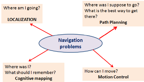
Robot Navigation involves all the related tasks and algorithms required to take a robot from point A to point B autonomously without any collisions. It is a well studied topic in Mobile Robotics, comprising volumes of books! The problem of Navigation is broken down into the following subproblems:

Localisation: The robot needs to know where it is.
Collision Avoidance: The robot needs to detect and avoid obstacles
Mapping: The robot needs to remember its surroundings
Planning: The robot needs to be able to plan a route to point B
Explore: The robot needs to be able to explore new terrain

Robot Navigation Problems

Some of the ways to achieve the task of Navigation are as follows:

Vision Based: Computer Vision algorithms and optical sensors, like LIDAR sensors are used for Vision Based Navigation.
Inertial Navigation: Airborne robots use inertial sensors for Navigation
Acoustic Navigation: Underwater robots use SONAR based Navigation Systems
Radio Navigation: Navigation used RADAR technology.

The problem of Path Planning in Navigation is dealt with in 2 ways, which are Global Navigation and Local Navigation

Global Navigation involves the use of a map of the environment to plan a path from point A to point B. The optimality of the path is decided based on the length of the path, the time taken to reach the target, using permanent roads etc. Global Positioning System (GPS) is one such example of Global Navigation. The algorithms used behind such systems may include Dijkstra, Best First or A* etc.

Once the global path is decided, it is broken down into suitable waypoints. The robot navigates through these waypoints in order to reach it’s destination. Local Navigation involves a dynamically changing path plan taking into consideration the changing surroundings and the vehicle constraints. Some examples of such algorithms would be Virtual Force Field, Follow Wall, Pledge Algorithm etc.

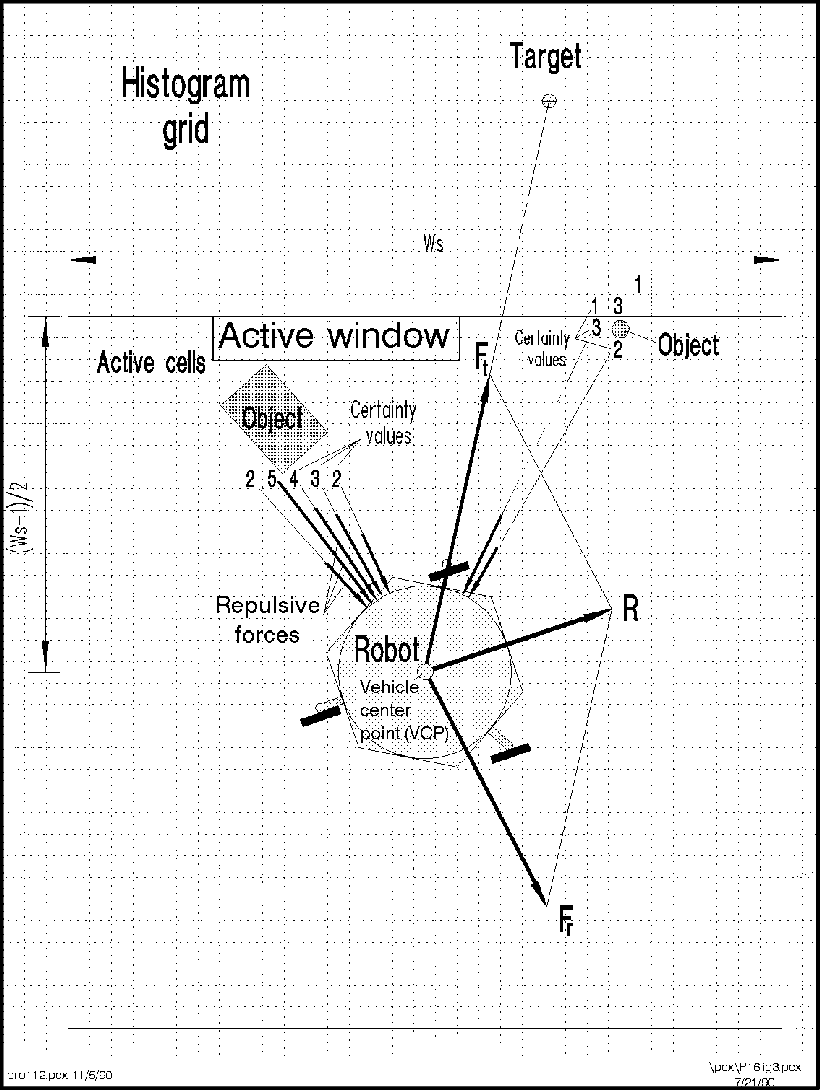
Virtual Force Field Algorithm

The Virtual Force Field Algorithm works in the following steps:

The robot assigns an attraction vector to the waypoint that points towards the waypoint.
The robot assigns a repulsion vector to the obstacle according to its sensor readings that points away from the waypoint. This is done by adding all the vectors that are translated from the sensor readings.
The robot follows the vector obtained by adding the target and obstacle vector.

VFF

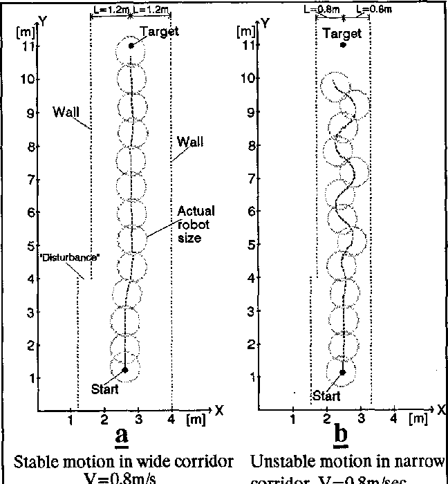
Drawbacks

There are a few problems related to this algorithm:

The robot tends to oscillate in narrow corridors, that is when the robot receives an obstacle vector simultaneously from opposite sides.
The robot may not be able to enter narrow corridors in the first place!

Drawbacks

Virtual Force Histogram Algorithm

This algorithm improves over the Virtual Force Field Algorithm, by using a data structure called the Polar Histogram. The robot maintains a histogram grid of the instantaneous sensor values received. Then, based on the threshold value set by the programmer, the program detects minimas(valleys) in the polar histogram. The angle corresponding to these values are then followed by the robot.

VFH

Note: The exercise only requires us to implement Virtual Force Field Algorithm

Hints

Simple hints provided to help you solve the local_navigation exercise. Please note that the full solution has not been provided.

Determining the Vectors

First of all, we need to generate the 3 required vectors, that are the Target Vector, Obstacle Vector and the Direction Vector.

Target Vector

The target vector can be easily obtained by subtracting the position of the car from the position of the next waypoint.

In order to implement this on the WebGUI interface of the exercise, in addition to the vector obtained by subtracting, we need to apply a rotation to the vector as well. The purpose of rotation is to keep the target vector always in the direction of the waypoint and not in front of the car. You may try seeing this in your own implementation, or refer to the illustrations

Refer to this webpage to know about the exact mathematical details of the implementation.

Obstacle Vector

The obstacle vector is to be calculated from the sensor readings we obtain from the surroundings of the robot. Each obstacle in front of the car, is going to provide a repulsion vector, which we will add to obtain the resulting repulsion vector. Assign a repulsion vector, for each of the 180 sensor readings. The magnitude of the repulsion vector is inversely proportional to the magnitude of the sensor reading. Once all the repulsion vectors are obtained, they are all added, to get the final one.

Note: There is a catch in this case, you may notice that most of the time in our implementation of the exercise we get an obstacle vector which is almost always pointing opposite to the direction in which we are supposed to head. This is a problem, as adding this vector directly to the target vector, would give a resulting vector which is more or less, quite not what we expected. Hence, there is a trick we need to apply to solve this problem.

_Obstacle Vector without any obstacles in front of the car*

Direction Vector

Conventionally and according to the research paper of the VFF algorithm, in order to obtain the direction vector we should add the target vector and the obstacle vector. But, due to an inherent problem behind the calculation of the obstacle vector, we cannot simply add them to obtain the final direction.

A simple observation reveals that we are required to keep moving forward for the purpose of this exercise. Hence, the component of the direction vector in the direction of motion of the car, has no effect on the motion of the car. Therefore, we can simply leave it as a constant, while adjusting the vector responsible for the steering of the car. It is the steering, that will in fact, provide us with the obstacle avoidance capabilities. Hence, the steering is going to be controlled by the Direction Vector.

Also, please note that this is not the only solution to this problem. We may also add an offset vector in the direction of motion of the car to cancel the effect of the redundant component.

Illustrations

examples — On applying the rotation matrix (left) - Without applying the rotation matrix (right)

Videos

Contributors

Contributors: Alberto Martín, Eduardo Perdices, Francisco Pérez, Victor Arribas, Julio Vega, Jose María Cañas, Nacho Arranz, Javier Izquierdo.
Maintained by Sakshay Mahna, Javier Izquierdo.

Goal

Frequency API

Python

C++

Robot API

HAL-based Implementation

Python

HAL-based Implementation

C++

ROS 2-direct Implementation

ROS 2 Topics

Python

C++

Conversion of types

Theory

Navigation

Global Navigation