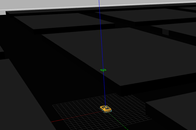
Global Navigation using TeleTaxi

Goal

The objective of this practice is to implement the logic of a Gradient Path Planning (GPP) algorithm. Global navigation through GPP, consists of:

Selected a destination, the GPP algorithm is responsible for finding the shortest path to it, avoiding, in the case of this practice, everything that is not road.
Once the path has been selected, the logic necessary to follow this path and reach the objective must be implemented in the robot.

With this, it is possible for the robot to go to the marked destination autonomously and following the shortest path.

The solution can integrate one or more of the following levels of difficulty, as well as any other one that occurs to you:

Reach the goal.
Optimize the way to find the shortest path.
Arrive as quickly as possible to the destination.

Instructions

This is the preferred way for running the exercise.

Installing and Launching

Download Docker. Windows users should choose WSL 2 backend Docker installation if possible, as it has better performance than Hyper-V.
Pull the current distribution of Robotics Academy Docker Image:
```
  docker pull jderobot/robotics-academy:latest
```

In order to obtain optimal performance, Docker should be using multiple CPU cores. In case of Docker for Mac or Docker for Windows, the VM should be assigned a greater number of cores.
It is recommended to use the latest image. However, older distributions of RADI (Robotics-Academy Docker Image) can be found here.

How to perform the exercises?

Start a new docker container of the image and keep it running in the background:

docker run --rm -it -p 7164:7164 -p 2303:2303 -p 1905:1905 -p 8765:8765 -p 6080:6080 -p 1108:1108 -p 7163:7163 jderobot/robotics-academy

On the local machine navigate to 127.0.0.1:7164/ in the browser and choose the desired exercise.
Wait for the Connect button to turn green and display “Connected”. Click on the “Launch” button and wait for some time until an alert appears with the message Connection Established and button displays “Ready”.
The exercise can be used after the alert.

Enable GPU Acceleration

Follow the advanced launching instructions from here.

Where to insert the code?

In the launched webpage, type your code in the text editor,

from GUI import GUI
from HAL import HAL
# Enter sequential code!


while True:
    # Enter iterative code!

Using the Interface

Control Buttons: The control buttons enable the control of the interface. Play button sends the code written by User to the Robot. Stop button stops the code that is currently running on the Robot. Save button saves the code on the local machine. Load button loads the code from the local machine. Reset button resets the simulation(primarily, the position of the robot).
Brain and GUI Frequency: This input shows the running frequency of the iterative part of the code (under the while True:). A smaller value implies the code runs less number of times. A higher value implies the code runs a large number of times. The numerator is the one set as the Measured Frequency who is the one measured by the computer (a frequency of execution the computer is able to maintain despite the commanded one) and the input (denominator) is the Target Frequency which is the desired frequency by the student. The student should adjust the Target Frequency according to the Measured Frequency.
RTF (Real Time Factor): The RTF defines how much real time passes with each step of simulation time. A RTF of 1 implies that simulation time is passing at the same speed as real time. The lower the value the slower the simulation will run, which will vary depending on the computer.
Pseudo Console: This shows the error messages related to the student’s code that is sent. In order to print certain debugging information on this console. The student can use the print() command in the Editor.

Robot API

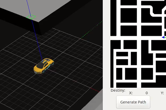
from HAL import HAL - to import the HAL(Hardware Abstraction Layer) library class. This class contains the functions that sends and receives information to and from the Hardware(Gazebo).
from GUI import GUI - to import the GUI(Graphical User Interface) library class. This class contains the functions used to view the debugging information, like image widgets.
from MAP import MAP - This class contains functions that interact with data related to the map and Gazebo world.
HAL.setV() - to set the linear speed
HAL.setW() - to set the angular velocity
HAL.getPose3d() - returns x,y and theta components of the robot in world coordinates
GUI.showNumpy(numpy) - shows Gradient Path Planning field on the user interface. It represents the values of the field that have been assigned to the array passed as a parameter. Accepts as input a two-dimensional uint8 numpy array whose values can range from 0 to 255 (grayscale). In order to have a grid with the same resolution as the map, the array should be 400x400
GUI.showPath(array) - shows a path on the map. The parameter should be a 2D array containing each of the points of the path
GUI.getTargetPose() - returns x,y coordinates of chosen destionation in the world. Destination is set by clicking on the map image
MAP.getMap(url) - - Returns a numpy array with the image data in grayscale as a 2 dimensional array. The URL of the Global Navigation map is ‘/RoboticsAcademy/exercises/static/exercises/global_navigation_newmanager/resources/images/cityLargenBin.png’, so the instruction to get the map is
```
array = MAP.getMap('/RoboticsAcademy/exercises/static/exercises/global_navigation_newmanager/resources/images/cityLargenBin.png')
```
MAP.rowColumn(vector) - returns the index in map coordinates corresponding to the vector in world coordinates passed as parameter

The map image has a resolution of 400x400 pixels and indicates wheter there is an obstacle or not by its color. The map in the Gazebo world has its center in [0, 0] and it has a width and height of 500 meters. Therefore, each of the pixels in the map image represent a cell in the Gazebo world with a width and height of 1.25 meters.

Videos

Theory

Motion Planning is a term used in robotics to find a sequence of valid configurations that moves the robot from source to destination. Motion Planning algorithms find themselves in a variety of settings, be it industrial manipulators, mobile robots, artificial intelligence, animations or study of biological molecules.

There are mainly 2 methods to solve the exercise, Gradient Path Planning, Sampling Based Path Planning

Gradient Path Planning

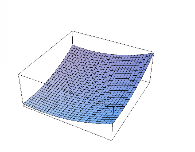
One such method for Motion Planning is Gradient Path Planning. GPP works on the principle of potential fields. The obstacles in the path serve as potential wall to the path planner, and the target serve as potential well. By combining all the potential walls and wells, a path is constructed as a downward slope. The robot follows that path to reach it’s destination.

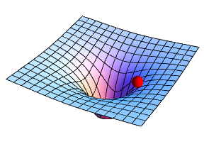
Potential Drop — Various illustrations based on potential

Potential Well — Various illustrations based on potential

Gradient Path Planning can be implemented using Brushfire Algorithm or Wave Front Algorithm. Next section explains the working of Wave Front Algorithm.

Wave Front Algorithm

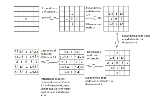
Wave Front Algorithm is BFS based approach to build a path from source to destination. The algorithm works by assigning weights to a grid of cells. Given the source and target, the algorithm starts from the target node and moves outwards like a ripple, while progressively assigning weights to the neighboring cells.

Assigning Weights

Assigning Weights

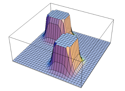
As for obstacles, additional weights are added to the cells that are close to obstacles. Intuitively, the weights represent the superposition of waves that are reflected from the walls of obstacles.

Superposition of Waves

Superposition of Waves

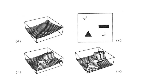
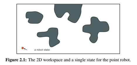
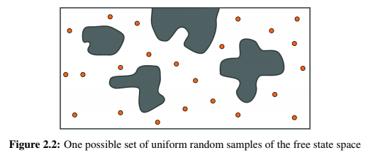
The algorithm stops upon reaching the source. To navigate through the generated path, the robot follows the path indicated by decreasing weights (a downhill drive). A grayscale image representation quite clearly depicts the path the robot might follow!

GrayScale Representation

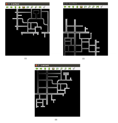
Gray Scale Representation

Sampling Based Path Planning

Sampling based Path Planning employs sampling of the state space of the robot in order to quickly and effectively plan paths, even with differential constraints or those with many degrees of freedom. Some of the algorithms under this class are:

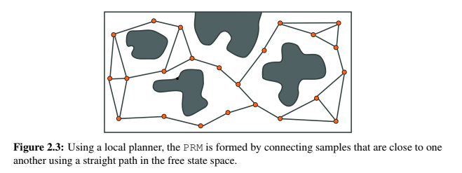
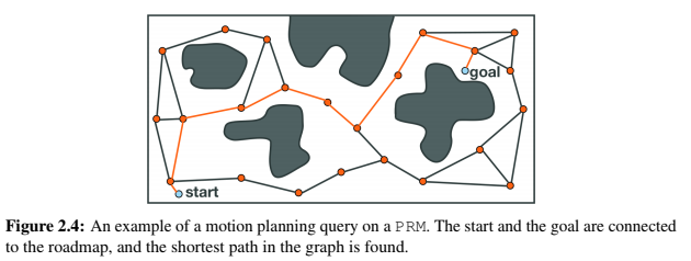
Probabilistic Roadmap

These methods work by randomly sampling points in the workspace. Once the desired number of samples are obtained, the roadmap is constructed by connecting the random samples to form edges. On the resulting graph formed, any shortest path algorithm (A*, Dijkstra, BFS) is applied to get our resulting path.

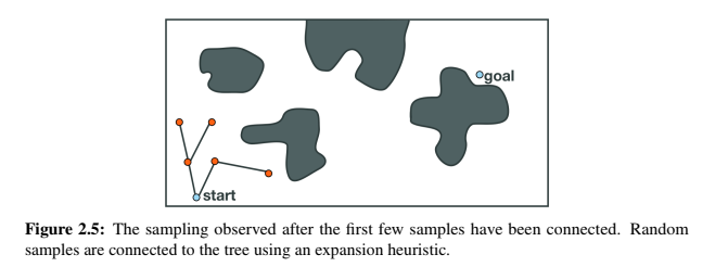
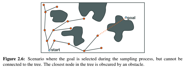
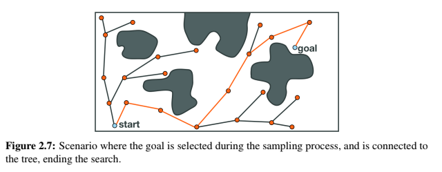
Tree Based Planner

Tree Based Planners are very similar to Probabilistic Roadmaps, except for the fact that there are no cycles involved in tree based planners. There are a variety of tree based planners, like RRT, EST, SBL and KPIECE. These algorithms work heuristically, working from the root node, a tree (a graph without cycles) is constructed.

Hints

Simple hints provided to help you solve the global navigation exercise. The hints are focused on solving the exercise through GPP algorithm.

Path Planning

Since, the map has already been divided into grids, we can directly work on the grid! Path Planning involves a BFS based search starting from the destination. The psuedo code for the algorithm is:

Step1: insert Target Node into priority queue
Step2: c = pop node from priority queue
Step3: if c == start node End
Step4: if c == obstacle Save to another list and goto Step2
Step5: assign weight to neighbors of c if previously unassigned
Step6: insert neighbors of c to priority queue
Step7: goto Step2

Assignment of weights to the cells is arbitrary. Generally, diagonally neighboring cells are assigned a greater weight than the other neighbors. Apart from all the assignment, the additional weight of cells close to obstacles is extremely important, as it is the one that is going to help avoid collisions!

Important Points to Remember

You may use MAP.getMap() to know whether an obstacle is present at (i, j) coordinate of the map. Also, in order to work with this grid, we have to invert our usage of coordinates. Implying, (i, j) can be accessed using (j, i).
In order to assign those extra weights, we may take the obstacle points we saved earlier, and add extra values to the neighbors of the obstacle cell afterwards.

The next step involves Path Navigation. We can start by defining the low level implementation like linear speed and angular speed. Using the orientation of the robot, distance and direction of the target, linear speed and angular speeds can be assigned to the robot.

For navigating effectively, we assign local goal points which eventually lead to the final destination. These local goal points can be selected by choosing 2 points, which occur one after the another recursively.

Also, make sure that the selection is done from a big enough radius, otherwise during navigation the robot may pass the grid and reach a local minima.