End to End Visual Control
Goal
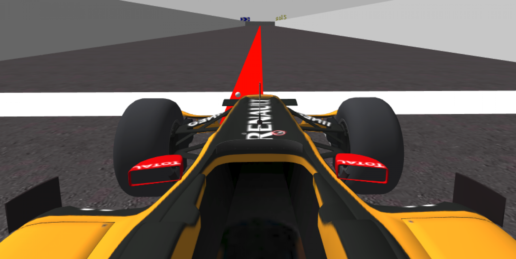
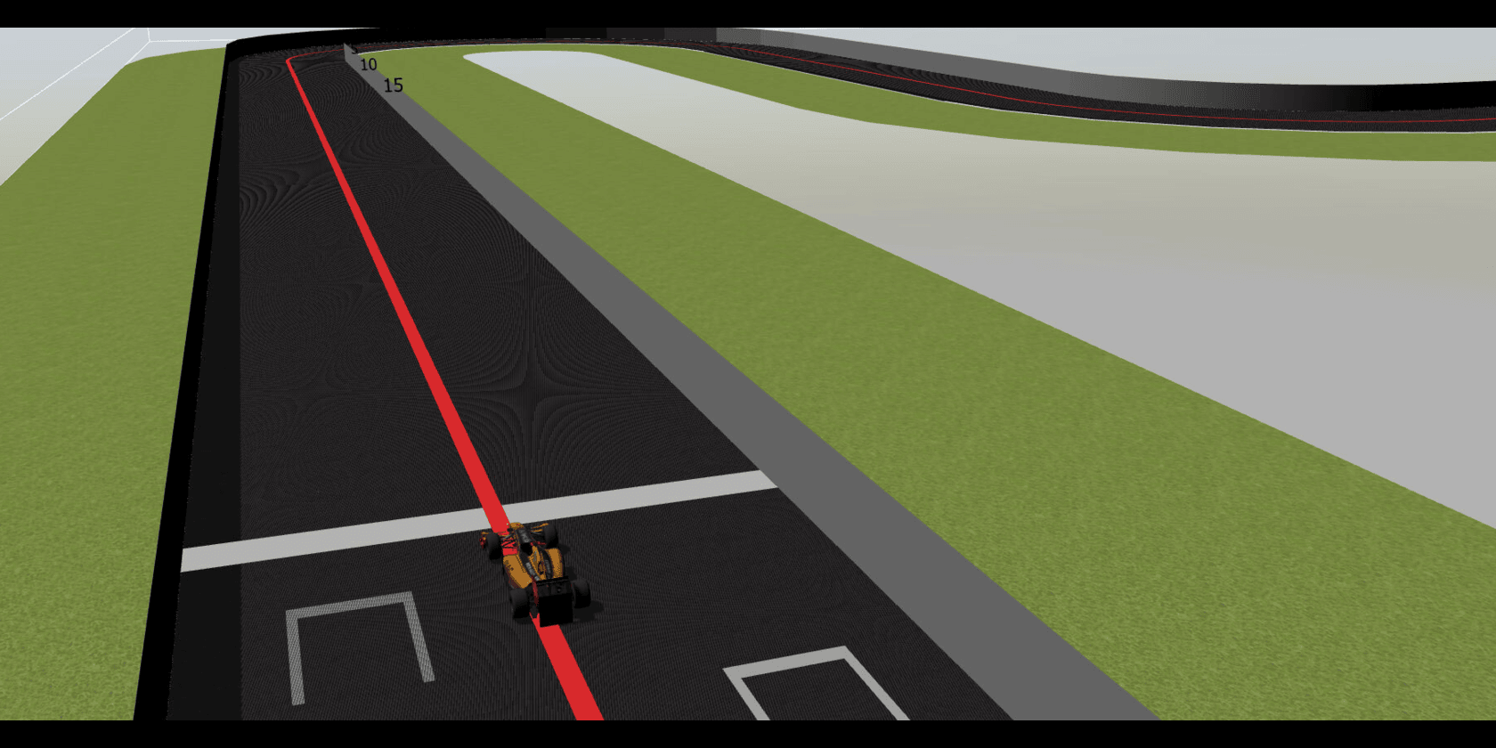
The end-to-end visual control exercise demonstrates end-to-end visual control of an autonomous vehicle using deep learning. The exercise provides datasets for students to develop and train their own deep learning models. The deep learning model takes raw images from the vehicle camera as input and predicts vehicle commands, including linear speed (v) and angular velocity (w), to navigate the autonomous vehicle through different circuits. Using the web interface, users can upload their models, test them in real-time inference, and observe how vision-based AI enables autonomous vehicle navigation within simulated environments created in Gazebo.
The students will develop a deep learning model that helps the autonomous vehicle complete the circuits.
🤖 Develop a Deep Learning Model
1. 💾 Dataset overview
For students who want to develop deep learning models for the End-to-End Visual Control exercise, we provide two datasets:
i) Simple Circuit Dataset
This dataset is specifically designed for training and testing models on a single, simple circuit. It is ideal for beginners or for initial experiments to understand how the model reacts to basic driving scenarios. The simple circuit is easier to complete, allowing users to quickly train and evaluate their models without facing complex turns or intersections.
ii) Combine Circuit Dataset
This dataset includes data from all four circuits available in the exercise. It is intended for advanced model development, enabling students to train models that generalize across all four circuits and handle various driving conditions, including sharp left and right turns. The combined dataset captures a wide range of driving scenarios, including sharp turns, straight paths, and varying circuit complexities. We provide an adjustment dataset designed to support users in managing diverse driving scenarios, facilitating more experimentation.
2. ☁️ Datasets Downloads
The datasets for the End-to-End Visual Control exercise are hosted on Huggingface under the JdeRobot organization. Students can access them using the load_dataset() method and directly apply them for training and testing their models. Although multiple download options are available, this guide highlights two recommended approaches for retrieving the datasets to a local machine.
Method 01: Use the git lfs command [Recommended: Low]
Visit the git-lfs website and install git-lfs on your local machine.
# Simple Circuit Dataset
git clone https://huggingface.co/datasets/JdeRobot/Follow-Line-Simple-Circuit-Dataset

# Combine Circuit Dataset
git clone https://huggingface.co/datasets/JdeRobot/Follow-Line-Combine-Dataset
Method 02: Huggingface Hub API [Recommended: High]
The Huggingface huggingface_hub library provides a Python API for interacting with the Huggingface Hub. The primary client class for this is HfApi, which lets you programmatically manage repositories, upload and download files, and access model metadata. The Hub also offers a free Inference API for running models directly on Huggingface.
First, create and activate a Python Environment⤴️ on your local machine and install the Huggingface Hub pip package. Next, obtain a Huggingface ACCESS TOKEN⤴️ from Huggingface and use it to download the datasets with code like:
Huggingface Hub Package
pip install huggingface_hub
Datasets Downloads code
from huggingface_hub import snapshot_download

# Download Simple Circuit Dataset to local folder
snapshot_download(repo_id="JdeRobot/Follow-Line-Simple-Circuit-Dataset",
    repo_type="dataset",resume_download=True,max_workers=16,
    token="HF_ACCESS_TOKEN",local_dir=output_dir
)

# Download Combine Dataset to local folder
snapshot_download(repo_id="JdeRobot/Follow-Line-Combine-Dataset",
    repo_type="dataset",resume_download=True,max_workers=16,
    token="HF_ACCESS_TOKEN",local_dir=output_dir
)
3. 📂 Datasets Folder Structure
Simple Circuit Dataset
The dataset is divided into training and testing parts. The training images are split into seven folders named train_images_part_01 to train_images_part_07, and their corresponding labels are provided in the train.csv file. For evaluation, the dataset includes a test_images folder that contains all the test images, with their labels stored separately in the test.csv file.
Combine Circuit Dataset
The dataset is organized into several folders and CSV files. The main training images are divided into six parts, stored in the folders images_part_01 to images_part_06. Each of these images is linked to labels provided in the train.csv file, which contains the vehicle commands. In addition to the main dataset, there is an adjustment_images folder that includes extra images intended for adjusting the sharp corner. The labels for these images are stored separately in the adjustment_data.csv file.
4. Model Training and Evaluation Pipeline
i) Data Preprocessing
Data preprocessing ensures that all inputs to the model are in a clean, consistent, and usable format. The Combine Circuit Dataset is already balanced.
However, the Simple Circuit Dataset is imbalanced. Training on such imbalanced data can cause the model to favor majority classes and perform poorly.
To address this, you should first categorize the samples into their respective classes and then apply data balancing techniques, such as:
- Undersampling: Reducing the number of majority-class samples.
- Oversampling: Increasing the number of minority-class samples, sometimes by duplicating or augmenting them.
In the preprocessing stage, images are first loaded from the dataset folders and paired with their corresponding labels from CSV files that contain control values such as linear and angular velocity. To ensure consistency, all images are resized to a fixed dimension and normalized by scaling pixel values to a standard range, which improves training stability. The labels are extracted directly from the CSV files and linked to the appropriate images. To enhance robustness and generalization, data augmentation techniques such as flipping, rotation, and brightness adjustment are applied, creating diverse variations of the training data.
ii) Dataset Splitting
The Simple Circuit dataset is divided into two sets: training and validation. The training set, which comprises the majority of the available data, is utilized to enable the model to learn underlying patterns and acquire the target task. The validation set is the data used during training to fine-tune hyper-parameters, prevent over-fitting, and monitor the model’s performance on unseen data.
The Combine Circuit Dataset consists of training data and adjustment data (used for sharp turns). If needed, these can be combined to create a larger dataset. You can then split the combined dataset into training and validation sets using an 80%-20% ratio with the train_test_split function (from sklearn.model_selection).
Example:
from sklearn.model_selection import train_test_split

# Combine training and adjustment data
all_data = train_data + adjustment_data

# Split into 80% train, 20% validation
train_set, val_set = train_test_split(all_data, test_size=0.2, random_state=42)
iii) Model Architecture and Training:
For this exercise, a deep learning model, such as a Convolutional Neural Network (CNN) like PilotNet or ResNet, can be chosen to perform End-to-End Visual Control. The model consists of multiple convolutional layers that automatically extract meaningful features from raw camera images, followed by fully connected layers that map these features to the predicted outputs, such as linear and angular velocities for the autonomous vehicle. As a starting point, users can also explore pretrained models provided by torchvision for experimentation and benchmarking.
During training, the model learns by comparing its predictions with the correct outputs (ground truth) from the dataset and trying to reduce the difference. This process uses backpropagation, which calculates how the model’s internal parameters (weights) should be adjusted to improve accuracy. Optimization algorithms like Adam are then applied to update these weights step by step. To make the model more reliable and avoid overfitting, techniques such as normalization, dropout, and adjustment of the learning rate may also be applied.
iv) Validation, Testing, and Evaluation:
While training, testing dataset is used to monitor the model’s performance on unseen data with the help of the Loss Validation graph. This helps ensure that the model is not just memorizing the training data (overfitting). Techniques such as early stopping (ending training when validation performance stops improving) or learning rate scheduling (gradually reducing the learning rate) may be applied to improve results.
Once training is complete, the model is evaluated on a testing dataset. To judge performance, different metrics could be used, such as Mean Squared Error (MSE), Mean Absolute Error (MAE), and the R-squared score for regression accuracy for classification tasks.
v) Export the Model
After training your deep learning model, you must export it to the ONNX (Open Neural Network Exchange)⤴️ format. This is the only model format currently supported by the RoboticsAcademy web interface. ONNX is an open standard that facilitates interoperability among various deep learning frameworks, including PyTorch and TensorFlow.
NB: RoboticsAcademy currently supports only the ONNX (Open Neural Network Exchange) format.
vi) Testing Criteria
While monitoring validation loss and checking evaluation metrics helps understand how well your model has learned, these measures do not guarantee that the autonomous vehicle can successfully complete a full circuit. To ensure real-world performance, you must also run the model in real-time inference within the End-to-End Visual Control exercise in the RoboticsAcademy environment and observe how it behaves while driving through the circuit.
| Dataset Name | Test Circuit | Result |
|---|---|---|
| Simple Circuit | Circuit Circuit only | A full lap must be completed on the Simple Circuit |
| Combine Circuit | All Four Circuits | A full lap must be completed within four circuits. |
Frequency API
import Frequency- to import the Frequency library class. This class contains the tick function to regulate the execution rate.Frequency.tick(ideal_rate)- regulates the execution rate to the number of Hz specified. Defaults to 50 Hz.
Robot API
This exercise now supports ROS 2-native implementation in addition to the original HAL-based approach. Below you’ll find the details for both options.
HAL-based Implementation
import HAL- to import the HAL (Hardware Abstraction Layer) library class. This class contains the functions that send and receive information to and from the Hardware (Gazebo).import WebGUI- to import the WebGUI (Web Graphical User Interface) library class. This class contains the functions used to view the debugging information, like image widgets.HAL.getImage()- to get the image (BGR8).HAL.setV(velocity)- to set the linear speed.HAL.setW(velocity)- to set the angular velocity.WebGUI.showImage(image)- allows you to view a debug image or with relevant information.
ROS 2-native Implementation
from WebGUI import gui - to enable the Web GUI for visualizing camera images.
Note: Ensure this import is included in your script to access the Web GUI functionalities.
ROS 2 Topics
Use standard ROS 2 topics for direct communication with the simulation.
/cam_f1_left/image_raw- Subscribe to this topic to receive camera images (BGR8). Message type:sensor_msgs/msg/Image/cmd_vel- Publish to this topic to set both linear and angular velocities. Message type:geometry_msgs/msg/Twist
Frequency Control
Use standard ROS 2 mechanisms to manage loop timing:
rclpy.spin()- Event-driven execution using callbacks.rclpy.spin_once()- Single-step processing, often with custom timers.rclpy.Rate()- Loop-based frequency control.
Image Debugging
- Publish processed images to the topic:
/webgui_imageUsed for sending debug or processed visuals to the frontend. - The GUI automatically subscribes to
/webgui_imageImages published to this topic are displayed in the GUI interface.
Run the Exercise
Enable GPU Acceleration
Deep learning models perform much faster when executed on a GPU compared to a CPU. To take advantage of GPU acceleration in this exercise, you need to ensure that your system has a compatible NVIDIA GPU and the required drivers installed⤴️.
RoboticsAcademy currently supports GPU acceleration on NVIDIA GPUs only. To take advantage of GPU support when running the RoboticsAcademy Docker image (RADI), you must use the provided execution script ⤴️.
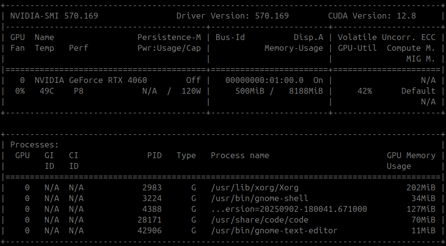
Verify GPU Availability
Run the following command to check if your GPU is accessible.
nvidia-smi
File Path for Uploaded Model
The model_path holds the file path to the uploaded ONNX model.
from model import model_path
Import GPU Configuration
ONNX Runtime supports running models on NVIDIA GPUs through the CUDA Execution Provider. This allows you to significantly speed up inference compared to CPU-only execution. import ONNX Runtime and preload the necessary CUDA/cuDNN libraries before creating a session:
import onnxruntime
from model import model_path

# Preload CUDA/cuDNN DLLs
onnxruntime.preload_dlls()

# Create an inference session that uses the GPU
session = onnxruntime.InferenceSession(
    model_path,
    providers=["CUDAExecutionProvider"] # CUDA as Execution provider
)
Debug
# To confirm that ONNX Runtime is using the GPU:
print("Execution Provider:", session.get_providers())

# Expected output should include:
['CUDAExecutionProvider', 'CPUExecutionProvider', ...]
Example Code
Recommended to load the ONNX model session
# Import the required package
from model import model_path
import onnxruntime
import sys

# preload dlls
onnxruntime.preload_dlls()

# Load ONNX model
try:
    ort_session = onnxruntime.InferenceSession(model_path,providers=["CUDAExecutionProvider"])
except Exception as e:
    print("ERROR: Model couldn't be loaded")
    print(str(e))
    sys.exit(1)
Exercise Instructions
- The uploaded ONNX format model should adhere to the input/output specifications, please keep that in mind while building your model.
- The user can train their model in any framework of their choice and export it to the ONNX format. Refer to this article to know more about exporting your model to the ONNX format.
References to ROS 2 Concepts
Understanding these ROS 2 concepts will help you implement the exercise natively. Refer to these links for more details:
- ROS 2 Publisher & Subscriber – https://docs.ros.org/en/humble/Tutorials/Beginner-Client-Libraries/Writing-A-Simple-Py-Publisher-And-Subscriber.html
- ROS 2 Spin & Spin Once – https://docs.ros.org/en/rolling/p/rclpy/api/init_shutdown.html
Videos
Demonstrative video of the solution
Contributors
- Contributors: Md. Shariar Kabir,Jose María Cañas,David Pascual, L. Roberto Morales
- Maintained by Md. Shariar Kabir,Jose María Cañas,David Pascual,L. Roberto Morales.